Contents
For a 10B parameter LLM, it requires ~176 GiB of GPU memory (FP32: 4 bytes/param, FP16: 2 bytes/param) for mixed precision training.
| Component | Precision | Explanation | Memory |
|---|---|---|---|
| Parameters / weights | bf16 | 10B * 2 bytes | 20 GB |
| Gradients | bf16 | 10B * 2 bytes | 20 GB |
| Optimizer states | fp32 | AdamW: momentum + variance 2 * (10B * 2 bytes) |
80 GB |
| FP32 master weights | fp32 | Used in mixed precision training 10B * 4 bytes |
40 GB |
| Activations | bf16 | Dependent on batch size & sequence length | ~20 GB |
| Temporary buffer | mixed | Attention, matmul, CUDA workspace (mixed) | ~10 GB |
| Total | 190 GB (~176 GiB) |
The A100 GPU has 80GB memory. Thus, distributed training is essential to train Large Language Models.
1. Background
There are two fundamental scaling approaches:
Horizontal Scaling (Scale Out)
- Add more machines/instances to distribute workload across smaller resources
- Easier to scale dynamically
- Requires more complex management
Vertical Scaling (Scale Up)
- Increase capacity of existing machine (more CPU, RAM, storage)
- Easier to manage
- Hardware upgrades can require downtime
In distributed training, we’re mainly working with horizontal scaling since machine specification is fixed e.g. p5.48xlarge AWS instance consists of 8xA100 GPUs with fixed memory and CPUs. And, also, a machine can only be scaled up to a point so we need to figure out to split our data or model on multiple GPUs machines. Distributed training is all about how to do that.
2. Communication Primitives
Before diving into parallelism strategies, it helps to understand the underlying communication operations.
Point-to-Point Communication
Direct transfer of data between two specific processes (send/receive).
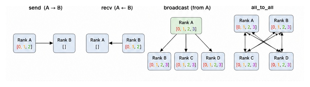
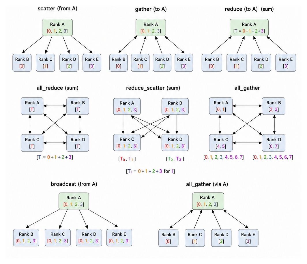
Collective Communication
Operations involving all processes in a group simultaneously.
3. Data Parallelism
Used when the model can fit in a single GPU. Each device (worker) holds a full copy of the model, but processes a different batch of training data. This way, data parallelism can scale up the training.
Data Parallelism Steps
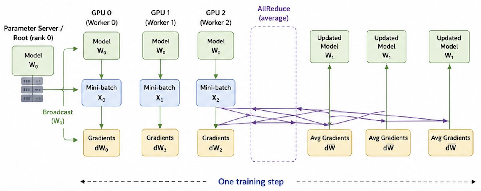
- Broadcast: Model weights are initialized on one GPU worker and broadcast to all other nodes.
- Forward pass: Each GPU worker has the same model (weights \(W\)) but processes different mini-batches \(X_i\).
- Backward pass: Each worker computes a weight gradient \(dW_i\) for its portion of weight parameters on local mini-batch.
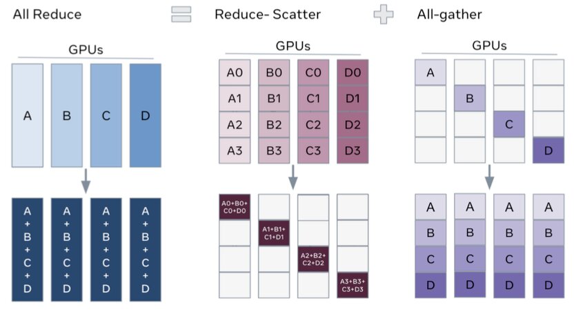
- Gradient synchronization: The gradients from each worker are averaged across all workers via
AllReduceoperation. Communication and computation can overlap with AllReduce gradients for layer \(k\) while computing gradients for layer \(k-1\). - Update: Each worker updates its local model parameters with the average gradients \(\overline{dW}\) using its own optimizer.
- \(\overline{dW} = (dW_0 + dW_1 + dW_3) / 3\), then
- \(W_1 = W - lr * \overline{dW}\).
- After the update, all workers have the same updated model weigths.
- Repeat: Go back to step 2 for next mini-batch.
The total global batch size is defined as the total records sent to all GPUs per iteration = (num of GPUs) × (per-replica batch size).
Parameter-server approach
An alternative approach for gradient synchronization is to use a separate server that stores parameters. In this setup, workers send gradients to parameter servers, the servers aggegrate the gradients and redistribute the model parameters.
Workers use a push-and-pull pattern:
- push gradients -> parameter server
- pull updated parameters <- parameter server
It can be synchronous (end of each training step) or asynchronous (replicas push/pull independently).
Key Points
- Data parallelism improve the overall throughput, but doesn’t reduce model memory per GPU.
- Each GPU worker processes roughly 1/N of global batch. However, each worker still stores the full model and performs full optimizer update for all parameters. Techniques like optimizer sharding, ZeRO, or FSDP can reduce this redundancy.
PyTorch Distributed Data Parallel (DDP)
The following code implements data parallelism with gradient accumulation:
def train():
    if global_rank == 0:
        initialize_services () # W&B, etc.
    data_loader = DataLoader(train_dataset, shuffle=False, sampler=DistributedSampler(train_dataset, shuffle=True))
    model = MyModel()
    if os path.exists('latest_checkpoint.pth'): # Load latest checkpoint
        # Also load optimizer state and other variables needed to restore the training state
        model. load_state_dict(torch.load('latest_checkpoint.pth'))
    model = DistributedDataParallel(model, device_ids=[local_rank])
    optimizer = torch.optim.Adam(model.parameters(), Ir=10e-4, eps=1e-9)
    loss_fn = torch.nn.CrossEntropyLoss()
    for epoch in range (num_epochs) :
        for data, labels in data_loader:
            if (step_number + 1) % 100 != 0 and not last_step: # Accumulate gradients for 100 steps
                with model.no_sync(): # Disable gradient synchronization
                    loss = loss_tn(model(data), labels) # Forward step
                    loss.backward() # Backward step + gradient ACCUMULATION
            else:
                loss = loss_fn(model(data), labels) # Forward step
                loss.backward() # Backward step + gradient SYNCHRONIZATION
                optimizer.step() # Update weights
                optimizer.zero_grad() # Reset gradients to zero
            if global_rank == 0:
                collect_statistics () # W&B, etc.
        if global_rank == 0: # Only save on rank o
            # Also save the optimizer state and other variables needed to restore the training state
            torch.save(model.state_dict(), "latest_checkpoint.pth')

if _name_ == '_main_':
    local_rank = int(os.environ['LOCAL_RANK' ])
    global_rank = int(os. environ ['RANK'])
    init_process_group (backend='nccl')
    torch.cuda.set_device(local_rank) # Set the device to local rank
    train()
    destroy_process_group()

# Run on all machines:
torchrun \
  --nnodes=NUM_NODES \
  --nproc-per-node=TRAINERS_PER_NODE \  # GPUs per node
  --max-restarts=NUM_ALLOWED_FAILURES \
  --rdzv-id=JOB_ID \
  --rdzv-backend=c10d \
  --rdzv-endpoint=HOST_NODE_ADDR \
  YOUR_TRAINING_SCRIPT.py [--arg1 ...]
4. Model Parallelism
Used when the model is too big to fit in a single GPU.
Pipeline Parallelism (Inter-layer)
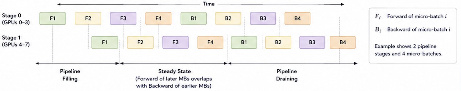
Pipeline parallelism partitions the model’s layers across multiple GPUs. The training mini-batch is split into micro-batches that flow through pipeline. The forward and backward computation of micro-batches are overlapped to reduce device idle time.
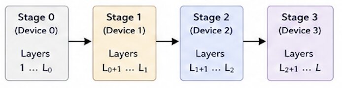
The pipeline parallelism on 4 stages on 4 GPU devices involves following steps.
- Partition model into 4 sequential stages and place each stage on a different device.
- Split global mini-batch into M micro-batches.
- Forward Pass:
- Pipeline Fill: Stage 0 on GPU 0 starts with micro-batch 0 and sends activations to Stage 1 on GPU 1. Each next stage starts when it receives activations.
- Steady State: All stages are busy. While Stage i works on micro-batch
k, Stagei-1can work on MBk+1. - Drain: The last stage finishes remaining micro-batches and computes the loss.
- Backward Pass (Drain → Fill): Gradients flow backward from Stage 3 to Stage 0 in the reverse order.
- Update Parameters: Each stage updates only its own parameters using the gradients it computed. Gradients are applied synchronously at the end.
- Repeat for the next global mini-batch.
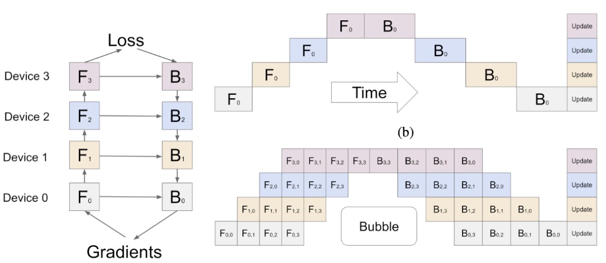
At the beginning, later stages are idle while the first micro-batch moves through pipeline. At the end, earlier stages become idle while the last backward computations finish. This idle time is called pipeline bubble. Increasing the number of micro-batches reduces the relative bubble overhead, but using too many can also increase scheduling complexity.
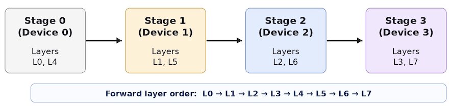
Interleaved Layers
In interleaved pipeline parallelism, non-contiguous layers (e.g., layer 1 and layer 4) are assigned to GPU workers instead of consecutive layers. This reduces worker idle time but increases communication overhead (worker communicates after every layer instead of every 2 layers). It’s can be complicated if model has skip connections, attention patterns that cross workers.
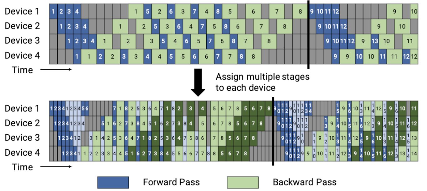
1F1B (One Forward, One Backward) Schedule
In classic data parallsielm, all micro-batches do all forward passes before any backward passes begin. In 1F1B:
Warm-up phase Workers perform differing numbers of forward passes.
Steady state Each worker performs one forward pass followed by one backward pass (unlike classic data parallelism where backward follows forward for all batches).
Drain phase Complete backward passes for all remaining in-flight micro-batches.
The default non-interleaved 1F1B has a smaller pipeline bubble than GPipe. The interleaved 1F1B (each device assigned multiple chunks) reduces the bubble size further.
Combining Pipeline Parallelism with Data Parallelism
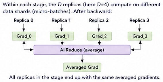
In this example, we split the model into 2 pipeline stages (Stage 0 and Stage 1). Each stage is replicated across 4 GPUs for data parallelism. Thus, total GPUs = 2 (pipeline) * 4 (data) = 8.
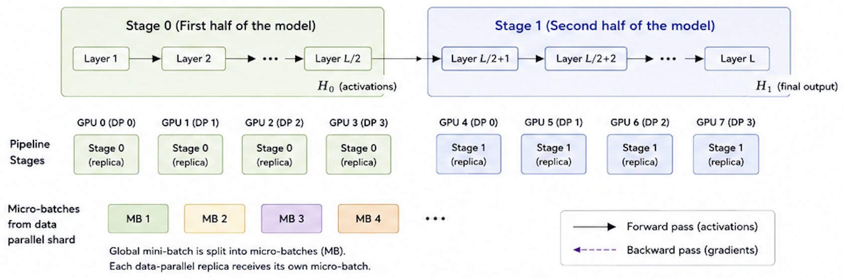
Here, the data parallel replicas are as of follows.
Pipeline replica Group 0:
GPU 0: Stage 0
GPU 4: Stage 1

Pipeline replica Group 1:
GPU 1: Stage 0
GPU 5: Stage 1

etc.
Pipeline Parallelism Steps:
- Split global mini-batch into M micro-batches.
- Each data-parallel in Stage 0 runs forward pass for its micro-batches.
- Activations are sent to Stage 1 replias; Stage 1 runs forward pass.
- After last stage produces outputs, backward pass flows from Stage 1 to Stage 0.
- Gradients are synchronized across data-parallel replicas within each stage using AllReduce.
- Optimizer updates are applied (per stage or globally, depending on setup).
- Repeat for next global mini-batch.
Tensor Parallelism (Intra-layer)
Tensor parallelism split the individual layer weights and computation across multiple GPUs unlike pipeline parallelism (which keeps individual weights intact but partitions layers). It’s required when a single parameter consumes most GPU memory, or for extremely large models like GPT.
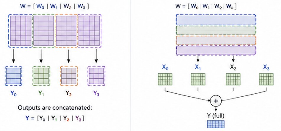
There are two ways to split the weight matrix W.
Column-wise Partitioning (by output dimension) No communication needed until a later layer requires the full output (then AllGather).
Row-wise Partitioning (by input dimension) Partial outputs are summed with AllReduce to get the full output.
Transformer MLP
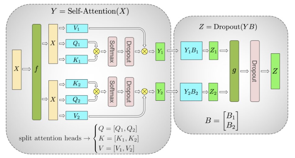
A Transformer MLP is usually. Y = GELU(XA); Z = YB.
In Megatron-LM tensor parallelism, the first GEMM weight matrix A is column-partitioned \(A = [A1, A2]\) so that GeLU nonlinearity can be applied independently to each partitioned GEMM output:
If we had split A into rows \(\begin{bmatrix}A1 \\ A2 \end{bmatrix}\), a sync point would have been needed since GeLU(X1A1 + X2A2) ≠ GeLU(X1A1) + GeLU(X2A2).
The second GEMM matrix B is row-partitioned \(\begin{bmatrix}B1 \\ B2 \end{bmatrix}\)
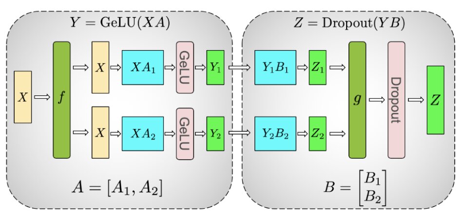
The advantage of partitioning the first MLP GEMM column-wise and the second MLP GEMM row-wise is that no communication is needed in-between until end of MLP blocks. An AllReduce is only needed after row-parallelism.
Note: Row-wise partitioning in the forward pass becomes column-wise partitioning in the backward pass and vice versa.
Multi-Head Attention (MHA)
MHA blocks are natural fit for tensor parallelism due to attention heads being mostly indpendent before final output projection. We can divide Q, K, V weight matrices by columns and the output linear layer by rows. This introduces two AllReduce operations per layer in both forward and backward passes.
5. Zero Redundancy Optimizer (ZeRO)
ZeRO consists of 3 stages which shards different model states: model parameters (weights), gradients, and optimizer states (e.g., momentum and variance in Adam).
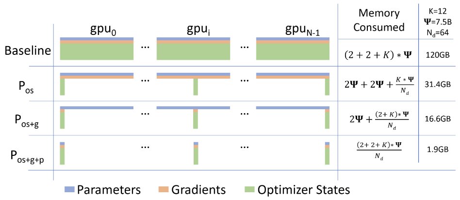
In the above figure, Ψ denotes model size (number of parameters), K denotes the memory multiplier of optimizer states, and Nd denotes data-parallel degree (#GPUs).
ZeRO Stage 1: Optimizer State Partitioning (Pos)
Shards optimizer states. Instead of creating per-param states for all parameters on every GPU, each optimizer instance only keeps states for a shard of all model parameters. The optimizer step() updates only its shard and then broadcasts updated parameters to all peers.
ZeRO Stage 2: Gradient Partitioning (Pos+g)
Shards both optimizer states and gradients across workers. Each worker maintains gradients only for its parameter partition. DeepSpeed performs a ReduceScatter (not AllReduce) so each worker only receives gradients for its own optimizer state partition.
With ZeRO Stage 1 and 2, the entire model must still fit on 1 GPU.
ZeRO Stage 3: Parameter Partitioning (Pos+g+p)
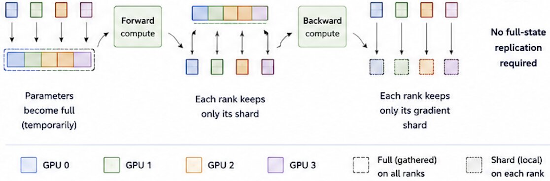
Shards all model states (optimizer, gradients, and model parameters). During computation, ZeRO 3 needs its full parameters so it temporarily gathers shards before a layer runs. Its working is quite similar to that of PyTorch FSDP.
Each GPU permanently stores only its own parameter shard, gradient shard, and optimizer shard. It gather the full parameters as needed and free them immediately after computation.


1 Before Forward: Each GPU holds only its parameter shards. Before forward pass, AllGather gets all parameters of layer, so every GPU has full parameters temporarily.
2 Forward Compute: Run forward with full parameters.
3 After Forward: Reshard (release) parameters to free memory.

4 Backward Compute: AllGather parameter shards again. Run backward pass to get local gradients.
5 After Backward: ReduceScatter gradients. Gradients are averaged across ranks, each rank keeps only its gradient shard.

6 Optimizer Step: Each rank updates its parameter shard using its optimizer state shard i.e. GPU 0 updates p0 shards, GPU 1 updates p1 shards, GPU 2 updates p2 shards using local optimizer-state shards.
ZeRO-Offload / ZeRO-Infinity:
ZeRO-Offload Offload optimizer states and gradients to CPU.
ZeRO Offload++ Offload optimizer and gradient states with better overlap.
ZeRO Infinity ZeRO-Offload + offload model weights to CPU/NVMe with better computation and communication overlap.
DeepSpeed Ulysses: Splits long sequence lengths across workers for sequence parallelism. Useful for long sequence length >10k.
DeepSpeed Training Setup
You can use Zero via DeepSpeed framework or use PyTorch FSDP for ZeRO Stage 3.
import deepspeed
ds_config = {
"train_batch_size": 32,
"gradient_accumulation_steps": 1,
"optimizer": {
"type": "Adam",
"params": {"lr": 3e-5}
},
"fp16": {"enabled": True},
"zero_optimization": {
"stage": 3, # ZeRO Stage 3
"offload_optimizer": {
"device": "cpu", # offload optimizer states to CPU
},
"offload_param": {
"device": "cpu", # offload parameters to CPU
},
"overlap_comm": True,
"contiguous_gradients": True,
"reduce_bucket_size": 5e8,
"stage3_prefetch_bucket_size": 5e7,
"stage3_param_persistence_threshold": 1e6,
},
}
model_engine, optimizer, _, _ = deepspeed.initialize(
model=model,
model_parameters=model.parameters(),
config=ds_config,
)
for batch in dataloader:
loss = model_engine(batch)
model_engine.backward(loss)
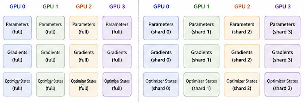
model_engine.step()6. PyTorch Fully Sharded Data Parallel (FSDP)
FSDP is a type of data-parallel training, but unlike traditional DDP (which maintains a per-GPU copy of model parameters, gradients, and optimizer states), FSDP shards all of these states across data-parallel workers and can optionally offload sharded parameters to CPU. It is effectively a mix of data and model parallelism. FSDP is PyTorch’s equivalent to DeepSpeed ZeRO Stage 3.
Advantages over DDP:
- Smaller GPU memory footprint → enables larger models or batch sizes.
- Communication overhead is reduced via overlapping communication and computation.
How FSDP Works
FSDP Forward Pass:
for layer_i in layers:
    all_gather full weights for layer_i   # reconstruct full weights from shards
    forward_pass(layer_i)
    discard full weights for layer_i      # free memory immediately
FSDP Backward Pass:
for layer_i in layers:
    all_gather full weights for layer_i
    backward_pass(layer_i)
    discard full weights for layer_i
    reduce_scatter gradients for layer_i  # average and reshard gradients
View as decomposed DDP: FSDP decomposes DDP’s gradient AllReduce into a ReduceScatter and an AllGather:
Backward pass Reduce-scatter gradients: each rank holds a shard of gradients.
Optimizer step Each rank updates its parameter shard.
Next forward pass AllGather to collect updated parameter shards.
Wrapping a Model with FSDP
Auto wrapping (drop-in DDP replacement):
from torch.distributed.fsdp import (
    FullyShardedDataParallel,
    CPUOffload,
)
from torch.distributed.fsdp.wrap import (
    default_auto_wrap_policy,
)
import torch.nn as nn

class MyModel(nn.Module):
    def __init__(self):
        super().__init__()
        self.layer1 = nn.Linear(8, 4)
        self.layer2 = nn.Linear(4, 16)
        self.layer3 = nn.Linear(16, 4)

# Replace DDP with FSDP:
# model = DistributedDataParallel(MyModel())
fsdp_model = FullyShardedDataParallel(
    MyModel(),
    fsdp_auto_wrap_policy=default_auto_wrap_policy,
    cpu_offload=CPUOffload(offload_params=True),
)
Manual wrapping allows selective application of FSDP to specific parts of the model for complex sharding strategies.
7. AWS SageMaker Distributed Training
The SageMaker API can be used for distributed training as follows.
SageMaker DDP (SMDDP)
from sagemaker.pytorch import PyTorch

estimator = PyTorch(
    ...,
    instance_count=2,
    instance_type="ml.p4d.24xlarge",
    # Option 1: mpirun with SMDDP AllReduce OR AllGather
    distribution={"pytorchddp": {"enabled": True}},
    # Option 2: torchrun, activates SMDDP AllGather
    # distribution={"torch_distributed": {"enabled": True}},
    # Option 3: mpirun with smddprun
    # distribution={"smdistributed": {"dataparallel": {"enabled": True}}},
)
For PyTorch DDP code, simply set the backend to smddp:
import torch.distributed as dist
import smdistributed.dataparallel.torch.torch_smddp

dist.init_process_group(backend="smddp")
SMDDP uses MPI (Message Passing Interface) for node communication and NVIDIA NCCL for GPU-level communication.
SageMaker Model Parallelism (SMP)
distribution = {
    "smdistributed": {
        "modelparallel": {
            "enabled": True,
            "parameters": {
                "hybrid_shard_degree": 2,          # degree of sharded data parallelism
                "sm_activation_offloading": True,   # offload activations to CPU
                "activation_loading_horizon": 4,
                "tensor_parallel_degree": 4,
                "expert_parallel_degree": 1,
                "random_seed": 42,
            },
        },
        "mpi": {"enabled": True},
    }
}
SMP provides Sharded data parallelism, Expert parallelism, Tensor parallelism, Activation checkpointing and offloading, etc funcationalities.
8. Summary: Parallelism Strategies
| Strategy | Splits | Use Case |
|---|---|---|
| Data Parallelism | Dataset across GPUs; full model replicated | Data doesn’t fit batch-wise on 1 GPU |
| Pipeline Parallelism | Layers across GPUs | Model layers don’t fit on 1 GPU |
| Tensor Parallelism | Individual weight tensors across GPUs | Single weights too large for 1 GPU |
| ZeRO / FSDP | Optimizer states, gradients, params sharded | Memory-efficient data parallelism |
| Hybrid | Combination of above | Very large models (GPT-3 scale and beyond) |
References and Image sources:
- Distributed communication package - torch.distributed
- GPipe: Easy Scaling with Micro-Batch Pipeline Parallelism
- PipeDream: Generalized Pipeline Parallelism for DNN Training
- Megatron-LM: Training Multi-Billion Parameter Language Models Using Model Parallelism
- ZeRO: Memory Optimizations Toward Training Trillion Parameter Models
- DeepSpeed ZeRO
- PyTorch FSDP
- PyTorch FSDP background