PyTorch libraries
- torchvision: for computer vision
- torchtext: for NLP
- torchaudio: for speech
PyTorch API (Python, C++, and CUDA)
- torch: core library
- torch.nn: for neural networks
- torch.nn.functional: defines functions
- torch.optim: for optimizers such as SGD
- C++
- ATen: foundational tensor operation library
- torch.autograd: for automatic differentiation
- torchscript: python to c++
- toch.onnx: for interoperatibility
Topics
- Immediate Vs Deferred execution modes
- Installation
- Tensors
- Autograd
- Data loading and augmentation
- Designing a neural network
- Transfer Learning
- Training, Validation, and Inference
- ONNX
- Assignment
Immediate Vs Deferred execution modes
PyTorch and Tensorflow 2 (by default) uses immediate (eager) mode. It follows the “define by run” principle i.e. you can execute the code as you define it. Consider the below simple example in Python.
a = 3
b = 4
c = (a**2 + b**2) ** 0.5
c
# 5.0
Tensorflow 1.0, on the other hand, uses deferred execution i.e. you define a series of operation first, then execute – most exceptions are be raised when the function is called, not when it’s defined. In the example below, a and b are placeholders, and the equation isn’t executed instantly to get the value of p unlike in immediate execution example above.
p = lambda a, b: (a**2 + b**2) ** 0.5
p(1, 2)
# 2.23606797749979
p(3, 4)
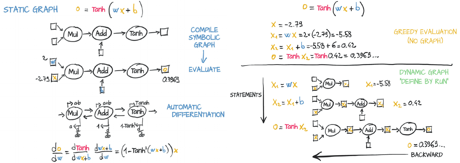
# 5.0In static graph (left side), the neuron gets compiled into a symbolic graph in which each node represents individual operations, using placeholders for inputs and outputs. Then the graph is evaluated numerically when numbers are plugged into the placeholders.
Dynamic graphs (righ side) can change during successive forward passes. Different nodes can be invoked according to conditions on the outputs of the preceding nodes, for example, without a need for such conditions to be represented in the graph.
Installation
I recommend creating a conda environment first. Then, follow the steps on PyTorch Getting Started. By default, the PyTorch library contains CUDA code, however, if you’re using CPU, you can download a smaller version of it.
# create conda env
conda create -n torchenv python=3.8
# activate env
conda activate torchenv
# install pytorch and torchvision
conda install pytorch torchvision cudatoolkit=10.1 -c pytorch
You can use collect_env.py script to test the installation.
Note: This tutorial works fine on PyTorch 1.4, torchvision 0.5.
Tensors
You can create and train neural networks in numpy as well. However, you won’t be able to use GPU, and will have to write the backward pass of gradient descent yourself, write your layers etc. The deep learning libraries, like PyTorch, solves all these types of problems. In short,
PyTorch = numpy with GPU + DL stuff
Note that in order to maintain reproducibility, you need to set both numpy and pytorch seeds.
import numpy as np
import torch

print(torch.__version__)

# reproducibility:  https://pytorch.org/docs/stable/notes/randomness.html
np.random.seed(0)
torch.manual_seed(7)
# when using CUDA and running on the CuDNN backend
torch.cuda.manual_seed_all(0)
torch.backends.cudnn.deterministic = True
torch.backends.cudnn.benchmark = False1.4.0A tensor is a generalization of matrices having a single datatype: a vector (1D tensor), a matrix (2D tensor), an array with three indices (3D tensor e.g. RGB color images). In PyTorch, similar to numpy, every tensor has a data type and can reside either on CPU or on GPU. For example, a tensor having 32-bit floating point numbers has data type of torch.float32 (torch.float). If the tensor is on CPU, it’ll be a torch.FloatTensor, and if on gpu, it’ll be a torch.cuda.FloatTensor. You can perform operations on these tensors similar to numpy arrays. In fact, PyTorch even has same naming conventions for basic functions as in numpy.
Read the complete list of types of tensors at PyTorch Tensor docs.
# uninitialized tensor
print(torch.empty(2, 2, dtype=torch.bool))

# initialized tensor
# torch.zeros(2, 2)
# torch.ones(2, 2)

print(torch.rand(2, 2))  # from a uniform distribution
print(torch.randn(2, 2)) # from standard normal distributiontensor([[True, True],
[True, True]])
tensor([[0.5349, 0.1988],
[0.6592, 0.6569]])
tensor([[ 0.9468, -1.1143],
[ 1.6908, -0.8948]])torch.Tensor is an alias for the default tensor type torch.FloatTensor.
# C, H, W
a = torch.Tensor(size=(3, 28, 28))
print(a.dtype, a.type(), a.shape)
# a.reshpae()
print(a.view(-1, 56).shape)torch.float32 torch.FloatTensor torch.Size([3, 28, 28])
torch.Size([42, 56])in-place operations
The in-place operations in PyTorch are those that directly modify the tensor content in-place i.e. without creating a new copy. The functions that have _ after their names are in-place e.g. add_() is in-place, while add() isn’t. Note that certain python operations such as a += b are also in-place.
a = torch.tensor([[1, 1], [1, 1]])
b = torch.tensor([[1, 1], [1, 1]])
# c = a + b  # normal operation
b.add_(a)  # in-place operation
print(b)tensor([[2, 2],
[2, 2]])np array <–> tensor
# tensor -> np array
b = b.numpy()
print(type(b))
# np array -> tensor
b = torch.tensor(b) # torch.from_numpy(b)
print(type(b))<class 'numpy.ndarray'>
<class 'torch.Tensor'>CUDA and GPU
# check if CUDA available
print(torch.cuda.is_available())
# check if tensor on GPU
print(b.is_cuda)
# move tensor to GPU
print(b.cuda()) # defaults to gpu:0 # or to.device('cuda')
# move tensor to CPU
print(b.cpu()) # or to.device('cpu')
# check tensor device
print(b.device)True
False
tensor([[2, 2],
[2, 2]], device='cuda:0')
tensor([[2, 2],
        [2, 2]])
cpuIf you’ve multiple GPUs, you can specify it using to.device('cuda:<n>). Here, n (0, 1, 2, …) denotes GPU number.
Autograd
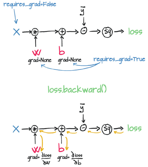
automatic differentiation: calculate the gradients of the parameters (W, b) with respect to the loss, L
It does so by keeping track of operations performed on tensors, then going backwards through those operations, calculating gradients along the way. For this, you need to set requires_grad = True on a tensor.
Consider the function z whose derivative w.r.t. x is x/2.
x = torch.randn(2,2, requires_grad=True)
y = x**2
# y.retain_grad()  # retain gradient
# each tensor has a .grad_fn attribute that references a Function that created it
print(f'y.grad_fn: {y.grad_fn}')
z = y.mean()

print(f'x.grad: {x.grad}')
z.backward()
print(f'x.grad: {x.grad}\n\
x/2: {x/2}\n\
y.grad: {y.grad}') # dz/dyy.grad_fn: <PowBackward0 object at 0x7f47f618c048>
x.grad: None
x.grad: tensor([[-0.0734, 0.3931],
[ 0.4734, -0.5572]])
x/2: tensor([[-0.0734, 0.3931],
[ 0.4734, -0.5572]], grad_fn=<DivBackward0>)
y.grad: NoneNote that the derivative of z w.r.t. y is None since gradients are calculated only for leaf variables by default.
You could use retain_grad() to calculate the gradient of non-left variables. You can use retain_graph=True so that the buffers are not freed. To reduce memory usage, during the .backward() call, all the intermediary results are deleted when they are not needed anymore. Hence if you try to call .backward() again, the intermediary results don’t exist and the backward pass cannot be performed.
z.backward()---------------------------------------------------------------------------
RuntimeError Traceback (most recent call last)
<ipython-input-9-40c0c9b0bbab> in <module>()
----> 1 z.backward()
/usr/local/lib/python3.6/dist-packages/torch/tensor.py in backward(self, gradient, retain_graph, create_graph)
193 products. Defaults to ``False``.
194 """
--> 195 torch.autograd.backward(self, gradient, retain_graph, create_graph)
196
197 def register_hook(self, hook):
/usr/local/lib/python3.6/dist-packages/torch/autograd/__init__.py in backward(tensors, grad_tensors, retain_graph, create_graph, grad_variables)
97 Variable._execution_engine.run_backward(
98 tensors, grad_tensors, retain_graph, create_graph,
---> 99 allow_unreachable=True) # allow_unreachable flag
100
101
RuntimeError: Trying to backward through the graph a second time, but the buffers have already been freed. Specify retain_graph=True when calling backward the first time.Note: Calling .backward() only works on scalar variables. When called on vector variables, an additional ‘gradient’ argument is required. In fact, y.backward() is equivalent to y.backward(torch.tensor(1.)). torch.autograd is an engine for computing vector-Jacobian product. Read more.
To stop a tensor from tracking history, you can call .detach() to detach it from the computation history, and to prevent future computation from being tracked OR use with torch.no_grad(): context manager.
print(x.requires_grad)
print((x ** 2).requires_grad)

with torch.no_grad():
    print((x ** 2).requires_grad)

print(x.requires_grad)
y = x.detach()
# best way to copy a tensor
# y = x.detach().clone()
print(y.requires_grad)
True
True
False
True
FalseNow, we’re going to train a simple dog classifier.
Data loading and augmentation
Dataset class is an abstract class representing a dataset.
ImageFolderrequires dataset to be in the format:root/dog/xxx.png root/dog/xxy.png root/dog/[...]/xxz.png root/cat/123.png root/cat/nsdf3.png root/cat/[...]/asd932_.png root/classname/image.png- Custom Dataset: It must inherit from Dataset class and override the
__len__so that len(dataset) returns the size of the dataset and__getitem__to support the indexing such thatdataset[i]can be used to getith sample.
In this tutorial, we’re going to use ImageFolder.
The DataLoader takes a dataset (such as you would get from ImageFolder) and returns batches of images and the corresponding labels.
We’re also going to normalize our input data and apply data augmentation techniques. Note that we don’t apply data augmentation to validation and testing split.
For nomalization, the mean and standard deviation should be taken from the training dataset, however, in this case, we’re going to use ImageNet’s statistics (why?).
import os
import PIL.Image
import numpy as np
import matplotlib.pyplot as plt

import torch
import torch.nn as nn
import torch.nn.functional as F
import torch.optim as optim
import torchvision
from torch.utils.data import Dataset, DataLoader
from torchvision import datasets, transforms
from torchvision.models import resnet101

%matplotlib inline
Get the dog breed classification dataset from Kaggle, Stanford Dog Dataset.
!wget https://s3-us-west-1.amazonaws.com/udacity-aind/dog-project/dogImages.zip
!unzip dogImages.zip
data_dir = 'dogImages'
data_transforms = {
'train': transforms.Compose([
transforms.RandomRotation(30),
transforms.RandomResizedCrop(224),
transforms.RandomHorizontalFlip(),
transforms.ToTensor(),
transforms.Normalize([0.485, 0.456, 0.406],
[0.229, 0.224, 0.225])
]),
'valid': transforms.Compose([
transforms.Resize(256),
transforms.CenterCrop(224),
transforms.ToTensor(),
transforms.Normalize([0.485, 0.456, 0.406],
[0.229, 0.224, 0.225])
]),
'test': transforms.Compose([
transforms.Resize(256),
transforms.CenterCrop(224),
transforms.ToTensor(),
transforms.Normalize([0.485, 0.456, 0.406],
[0.229, 0.224, 0.225])
]),
}
print("Initializing Datasets and Dataloaders...")
image_datasets = {x: datasets.ImageFolder(os.path.join(data_dir, x),
data_transforms[x])
for x in ['train', 'valid', 'test']}
# image, label
loaders = {x: DataLoader(image_datasets[x], batch_size=32,
shuffle=True)
for x in ['train', 'valid', 'test']}
dataset_sizes = {x: len(image_datasets[x]) for x in ['train', 'valid', 'test']}
print(dataset_sizes)
class_names = image_datasets['train'].classes
n_classes = len(class_names)
n_classesInitializing Datasets and Dataloaders...
{'train': 6680, 'valid': 835, 'test': 836}
133use_cuda = torch.cuda.is_available()
device = torch.device("cuda:0" if torch.cuda.is_available() else "cpu")
devicedevice(type='cpu')Designing a neural network
There are two ways we can implement different layers and functions in PyTorch. torch.nn module (python class) is a real layer which can be added or connected to other layers or network models. However, torch.nn.functional (python function) contains functions that do some operations, not the layers which have learnable parameters such as weights and bias terms. Still, the choice of using torch.nn or torch.nn.functional is yours. torch.nn is more convenient for methods which have learnable parameters. It keep the network clean.
Note: Always use nn.Dropout(), not F.dropout(). Dropout is supposed to be used only in training mode, not in evaluation mode, nn.Dropout() takes care of that.
The spatial dimensions of a convolutional layer can be calculated as: (W_in−F+2P)/S+1, where W_in is input, F is filter size, P is padding, S is stride.
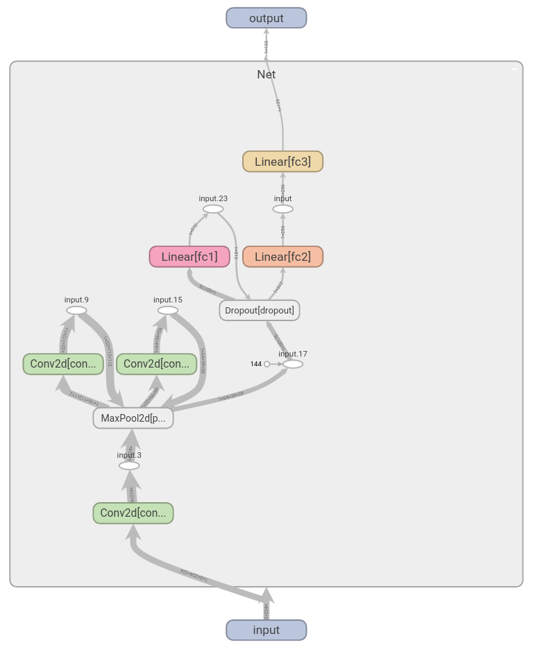
class Net(nn.Module):
    def __init__(self):
        super(Net, self).__init__()
        # input image: (3, 224, 224)
        self.conv1 = nn.Conv2d(in_channels=3, out_channels=16, kernel_size=3, padding=1)
        # (16, 224, 224) --> (16, 112, 112) (halved by max-pool)
        self.conv2 = nn.Conv2d(16, 32, 3, padding=1)
        # (32, 56, 56)
        self.conv3 = nn.Conv2d(32, 64, 3, padding=1)
        self.pool = nn.MaxPool2d(2, 2)
        # (64, 28, 28)
        self.fc1 = nn.Linear(64*28*28, 512)
        self.fc2 = nn.Linear(512, 256)
        # no of classes `n_classes`: 133
        self.fc3 = nn.Linear(256, n_classes)
        self.dropout = nn.Dropout(0.25)

    def forward(self, x):
        ## forward pass
        x = self.pool(F.relu(self.conv1(x)))
        x = self.pool(F.relu(self.conv2(x)))
        x = self.pool(F.relu(self.conv3(x)))
        # flatten image input
        x = x.view(-1, 64 * 28 * 28)
        x = self.dropout(x)
        x = F.relu(self.fc1(x))
        x = self.dropout(x)
        x = F.relu(self.fc2(x))
        x = self.fc3(x)
        return x

# instantiate the CNN
model_scratch = Net()

# move tensors to GPU if CUDA is available
model_scratch = model_scratch.to(device)

print(model_scratch)Net(
(conv1): Conv2d(3, 16, kernel_size=(3, 3), stride=(1, 1), padding=(1, 1))
(conv2): Conv2d(16, 32, kernel_size=(3, 3), stride=(1, 1), padding=(1, 1))
(conv3): Conv2d(32, 64, kernel_size=(3, 3), stride=(1, 1), padding=(1, 1))
(pool): MaxPool2d(kernel_size=2, stride=2, padding=0, dilation=1, ceil_mode=False)
(fc1): Linear(in_features=50176, out_features=512, bias=True)
(fc2): Linear(in_features=512, out_features=256, bias=True)
(fc3): Linear(in_features=256, out_features=133, bias=True)
(dropout): Dropout(p=0.25, inplace=False)
)# !pip install torchsummary
from torchsummary import summary
summary(model_scratch, input_size=(3, 224, 224))----------------------------------------------------------------
Layer (type) Output Shape Param #
================================================================
Conv2d-1 [-1, 16, 224, 224] 448
MaxPool2d-2 [-1, 16, 112, 112] 0
Conv2d-3 [-1, 32, 112, 112] 4,640
MaxPool2d-4 [-1, 32, 56, 56] 0
Conv2d-5 [-1, 64, 56, 56] 18,496
MaxPool2d-6 [-1, 64, 28, 28] 0
Dropout-7 [-1, 50176] 0
Linear-8 [-1, 512] 25,690,624
Dropout-9 [-1, 512] 0
Linear-10 [-1, 256] 131,328
Linear-11 [-1, 133] 34,181
================================================================
Total params: 25,879,717
Trainable params: 25,879,717
Non-trainable params: 0
----------------------------------------------------------------
Input size (MB): 0.57
Forward/backward pass size (MB): 13.79
Params size (MB): 98.72
Estimated Total Size (MB): 113.09
----------------------------------------------------------------
Transfer Learning
PyTorch transfer learning offical tutorial
Instead of training the model we created from scratch, we’re going to fine-tune pretrained model.
model_transfer = resnet101(pretrained=True)
print(model_transfer)
The classifier part of the model is a single fully-connected layer (fc): Linear(in_features=2048, out_features=1000, bias=True). This layer was trained on the ImageNet dataset, so it won’t work for our specific problem, so we need to replace the classifier.
# Freeze parameters so we don't backprop through them
for param in model_transfer.parameters():
    param.requires_grad = False

num_ftrs = 2048 #model_transfer.fc.in_features  # it's 2048, check fc layer of resnet

# creating model using Sequential API
classifier = nn.Sequential(nn.Linear(num_ftrs, 512),
                           nn.ReLU(),
                           nn.Dropout(0.2),
                           nn.Linear(512, 133))
model_transfer.fc = classifier

model_transfer = model_transfer.to(device)
print(model_transfer)
summary(model_transfer, input_size=(3, 224, 224))
Training, Validation, and Inference
Since, it’s a classification problem, we’ll use cross-entropy loss function.
\[\text{Cross-entropy} = -\sum_{i=1}^n \sum_{j=1}^m y_{i,j}\log(p_{i,j})\]where, \(y_{i,j}\) denotes the true value i.e. 1 if sample i belongs to class j and 0 otherwise, and \(p_{i,j}\) denotes the probability predicted by your model of sample i belonging to class j.
nn.CrossEntropyLoss() combines nn.LogSoftmax() (log(softmax(x))) and nn.NLLLoss() (negative log likelihood loss) in one single class. Therefore, the output from the network that is passed into nn.CrossEntropyLoss needs to be the raw output of the network (called logits), not the output of the softmax function.
It is convenient to build the model with a log-softmax output using nn.LogSoftmax (or F.log_softmax) since the actual probabilities can be accessed by taking the exponential torch.exp(output), then negative log likelihood loss, nn.NLLLoss can be used. Read more.
criterion = nn.CrossEntropyLoss() # LogSoftmax + NLLLoss
# only train the classifier (fully-connected layers') parameters
optimizer = optim.Adam(model_transfer.fc.parameters(), lr=0.001)- one epoch = one forward pass and one backward pass of all the training examples.
- batch size = the number of training examples in one forward/backward pass. The higher the batch size, the more memory space you’ll need.
- number of iterations = number of passes, each pass using [batch size] number of examples. To be clear, one pass = one forward pass + one backward pass (we do not count the forward pass and backward pass as two different passes).
Example: if you have 1000 training examples, and your batch size is 4, then it will take 250 iterations to complete 1 epoch.
Note: the weights are updated after each batch, not epoch or iteration.
Calling backward leads derivatives to accumulate at leaf nodes. You need to zero the gradient explicitly after using it for parameter updates i.e. optimizer.zero_grad(). We can utilize this functionality to Increase effective batch size using gradient accmulation
def train(n_epochs, loaders, model, optimizer, criterion, use_cuda, save_path):
    """returns trained model"""
    # initialize tracker for minimum validation loss
    valid_loss_min = np.Inf

    for epoch in range(1, n_epochs+1):
        # initialize variables to monitor training and validation loss
        train_loss = 0.0
        valid_loss = 0.0

        ###################
        # train the model #
        ###################
        model.train()
        for batch_idx, (data, target) in enumerate(loaders['train']):
            # move to GPU, if available
            # image, label
            if use_cuda:
                data, target = data.cuda(), target.cuda() # .to(device)
            # zero the parameter gradients
            optimizer.zero_grad()
            # forward pass: compute predicted outputs by passing inputs to the model
            # [N, C, H, W] -> [32, 3, 224, 224]
            outputs = model(data)
            # calculate the loss
            loss = criterion(outputs, target)
            # backward pass
            loss.backward()
            # optimization step (update the weights)
            optimizer.step()
            # record the average training loss
            # train_loss += loss.item()*data.size(0)
            # if using above method then divide loss "outside this for-loop":
            # using this (to get epoch loss): train_loss = train_loss/len(loaders['train'])
            train_loss += ((1 / (batch_idx + 1)) * (loss.data - train_loss))

        ######################
        # validate the model #
        ######################
        # set model to evaluation model (disables dropout etc)
        model.eval()
        for batch_idx, (data, target) in enumerate(loaders['valid']):
            if use_cuda:
                data, target = data.cuda(), target.cuda()
            # Turn off gradients for validation, saves memory and computations
            with torch.no_grad():
                outputs = model(data)
                loss = criterion(outputs, target)
                valid_loss += ((1 / (batch_idx + 1)) * (loss.data - valid_loss))


        # print training/validation statistics
        print('Epoch: {} \tTraining Loss: {:.6f} \tValidation Loss: {:.6f}'.format(
            epoch,
            train_loss,
            valid_loss
            ))

        ## serialization: save the model if validation loss has decreased
        if valid_loss <= valid_loss_min:
            print(f'Validation loss decreased ({valid_loss_min:.3f} --> {valid_loss:.3f}).  Saving model ...')
            torch.save(model.state_dict(), save_path)
            valid_loss_min = valid_loss

    return model
from PIL import ImageFile
ImageFile.LOAD_TRUNCATED_IMAGES = True# train the model
model_transfer = train(5, loaders, model_transfer, optimizer, criterion, use_cuda, 'model_transfer.pt')Epoch: 1 Training Loss: 2.871226 Validation Loss: 1.018821
Validation loss decreased (inf --> 1.019). Saving model ...
Epoch: 2 Training Loss: 1.468614 Validation Loss: 0.654094
Validation loss decreased (1.019 --> 0.654). Saving model ...
Epoch: 3 Training Loss: 1.249909 Validation Loss: 0.551980
Validation loss decreased (0.654 --> 0.552). Saving model ...
Epoch: 4 Training Loss: 1.162452 Validation Loss: 0.498752
Validation loss decreased (0.552 --> 0.499). Saving model ...
Epoch: 5 Training Loss: 1.122475 Validation Loss: 0.470465
Validation loss decreased (0.499 --> 0.470). Saving model ...# load the model that got the best validation accuracy (uncomment the line below)
# model_transfer.load_state_dict(torch.load('model_transfer.pt'))The .parameters() only gives the module parameters i.e. weights and biases, while state_dict returns a dictionary containing a whole state of the module.
for name, param in model_scratch.named_parameters():
    if param.requires_grad:
print(name)conv1.weight
conv1.bias
conv2.weight
conv2.bias
conv3.weight
conv3.bias
fc1.weight
fc1.bias
fc2.weight
fc2.bias
fc3.weight
fc3.biasmodel_transfer.state_dict().keys()odict_keys(['conv1.weight', 'bn1.weight', 'bn1.bias', 'bn1.running_mean', 'bn1.running_var', 'bn1.num_batches_tracked', 'layer1.0.conv1.weight', 'layer1.0.bn1.weight', 'layer1.0.bn1.bias', 'layer1.0.bn1.running_mean', 'layer1.0.bn1.running_var', 'layer1.0.bn1.num_batches_tracked', 'layer1.0.conv2.weight', 'layer1.0.bn2.weight', 'layer1.0.bn2.bias', 'layer1.0.bn2.running_mean', 'layer1.0.bn2.running_var', 'layer1.0.bn2.num_batches_tracked', 'layer1.0.conv3.weight', 'layer1.0.bn3.weight', 'layer1.0.bn3.bias', 'layer1.0.bn3.running_mean', 'layer1.0.bn3.running_var', 'layer1.0.bn3.num_batches_tracked', 'layer1.0.downsample.0.weight', 'layer1.0.downsample.1.weight', 'layer1.0.downsample.1.bias', 'layer1.0.downsample.1.running_mean', 'layer1.0.downsample.1.running_var', 'layer1.0.downsample.1.num_batches_tracked', 'layer1.1.conv1.weight', 'layer1.1.bn1.weight', 'layer1.1.bn1.bias', 'layer1.1.bn1.running_mean', 'layer1.1.bn1.running_var', 'layer1.1.bn1.num_batches_tracked', 'layer1.1.conv2.weight', 'layer1.1.bn2.weight', 'layer1.1.bn2.bias', 'layer1.1.bn2.running_mean', 'layer1.1.bn2.running_var', 'layer1.1.bn2.num_batches_tracked', 'layer1.1.conv3.weight', 'layer1.1.bn3.weight', 'layer1.1.bn3.bias', 'layer1.1.bn3.running_mean', 'layer1.1.bn3.running_var', 'layer1.1.bn3.num_batches_tracked', ...])torch.nn only supports mini-batches. For example, nn.Conv2d will take in a 4D Tensor of NCHW (nSamples x nChannels x Height x Width) .If you have a single sample, just use input.unsqueeze(0) to add a fake batch dimension.
class_names = [item[4:].replace("_", " ") for item in image_datasets['train'].classes]
loader_transform = data_transforms['test']

def predict_breed_transfer(img_path):
    img = PIL.Image.open(img_path)
    plt.imshow(img)
    plt.axis('off')
    plt.show()
    img = loader_transform(img).float()
    # 3, 224, 224
    img = img.unsqueeze(0)  # Add batch size for PyTorch: [N, C, H, W]: [1, 3, 224, 224]
    model_transfer.cpu()
    _, preds = torch.max(model_transfer(img), 1)
    return class_names[preds]

predict_breed_transfer('dogImages/train/001.Affenpinscher/Affenpinscher_00001.jpg')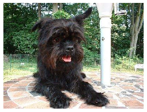
'Affenpinscher'ONNX
- ONNX (Open Neural Network Exchange) is an open format to represent models thus allowing interoperability.
- It defines a common set of operators (opsets) that a model uses and creates
.onnxmodel file that can be converted to various frameworks.
device = torch.device("cuda:0" if torch.cuda.is_available() else "cpu")
print('Using', device)

batch_size = 1  # just take random number
dummy_input = torch.randn(batch_size, 3, 224, 224)

# move model to gpu if available
model_transfer.to(device)
# set eval mode
model_transfer.eval()
# move input to gpu if available
dummy_input = dummy_input.to(device)
# output using pytorch
torch_out = model_transfer(dummy_input)
# print('torch_out', torch_out)
print('shape:', torch_out.shape)

# export the model
torch.onnx.export(model_transfer,             # model being run
                 dummy_input,                 # model input (or a tuple for multiple inputs)
                 'resnet101.onnx',            # where to save the model (can be a file or file-like object)
                 input_names = ['input_1'],   # the model's input names
                 output_names = ['output_1'], # the model's output names
                 dynamic_axes={'input_1' : {0 : 'batch_size'},   # variable length axes
                               'output_1' : {0 : 'batch_size'}})

print('Model exported successfully!')
Using cuda:0
shape: torch.Size([1, 1000])
Model exported successfully!# !pip install onnx onnxruntime-gpu
import onnx, onnxruntime
model_name = 'resnet101.onnx'
onnx_model = onnx.load(model_name)
onnx.checker.check_model(onnx_model)
ort_session = onnxruntime.InferenceSession(model_name)
def to_numpy(tensor):
return tensor.detach().cpu().numpy() if tensor.requires_grad else tensor.cpu().numpy()
# compute ONNX Runtime output prediction
ort_inputs = {ort_session.get_inputs()[0].name: to_numpy(dummy_input)}
ort_outs = ort_session.run(None, ort_inputs)
# compare ONNX Runtime and PyTorch results
print('ort_outs[0]: ', ort_outs[0].shape)
np.testing.assert_allclose(to_numpy(torch_out), ort_outs[0], rtol=1e-03, atol=1e-05)
print("Exported model has been tested with ONNXRuntime, and the result looks good!")ort_outs[0]: (1, 1000)
Exported model has been tested with ONNXRuntime, and the result looks good!Assignment
Assignment 1
- Calculate the second derivative of
x^2+x. - Create a custom layer that perform convolution then optional batch normalization.
ConvWithBatchNorm(in_channels=3, out_channels=16, kernel_size=4, stride=2, padding=1, batch_norm=False) - Initialize the weights of a single linear layer from a uniform distribution.
- Calculate cross-entropy loss for the following:
Note thatcross_entropyornll_lossin pytorch takes the raw inputs, not probabilites while calculating loss.
(4a).labels: [1, 0, 2] logits = [2.5, -0.5, 0.1], [-1.1, 2.5, 0.0], [1.2, 2.2, 3.1](4b).
labels: [1, 0, 1] probabilites: [0.1, 0.9], [0.9, 0.1], [0.2, 0.8] - Fix the below code to create a model having multiple linear layers:
class MyModule(nn.Module):
 def __init__(self):
     super(MyModule, self).__init__()
     self.linears = []
     for i in range(5):
         self.linears.append(nn.Linear(10, 10))

 def forward(self, x):
     for i, l in enumerate(self.linears):
         x = self.linears[i // 2](x) + l(x)
     return x
model = MyModule()
print(model)
Assignment 2
- Use Transfer Learning to fine-tune the model on the following dataset and achieve validation classification accuracy of at least 0.85 (or validation loss 0.25) during training. (Choose pretrained model of your choice.)
Dataset: Flower images [Read more here]
Note: Don’t forget to normalize the data before training. You can also apply data augmentation, regularization, learning rate decay etc.
QUIZ: Test Your Knowledge
Special thanks to Udacity, where I started my PyTorch journey through PyTorch Scholarship and Deep Learning Nanodegree.
If you’re looking for more PyTorch basic projects. Check kHarshit/udacity-nanodegree-projects.
Resources
Comments