This is the third post in the Quick intro series: object detection (I), semantic segmentation (II).

“Boxes are stupid anyway though, I’m probably a true believer in masks except I can’t get YOLO to learn them.” — Joseph Redmon, YOLOv3

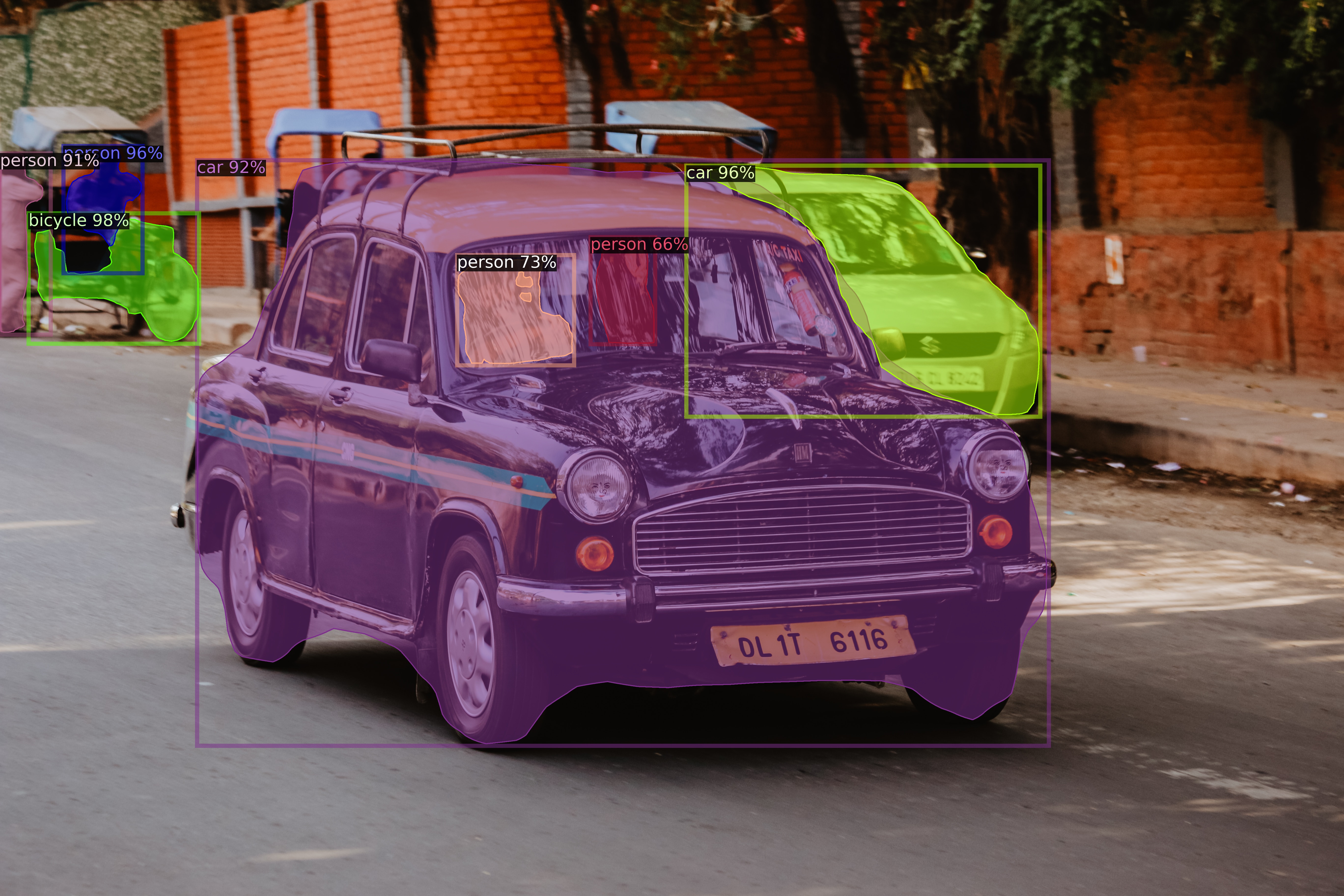
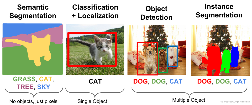
The instance segmentation combines object detection, where the goal is to classify individual objects and localize them using a bounding box, and semantic segmentation, where the goal is to classify each pixel into the given classes. In instance segmentation, we care about detection and segmentation of the instances of objects separately.

Mask R-CNN

Mask R-CNN is a state-of-the-art model for instance segmentation. It extends Faster R-CNN, the model used for object detection, by adding a parallel branch for predicting segmentation masks.

Before getting into Mask R-CNN, let’s take a look at Faster R-CNN.

Faster R-CNN

Faster R-CNN consists of two stages.

Stage I

The first stage is a deep convolutional network with Region Proposal Network (RPN), which proposes regions of interest (ROI) from the feature maps output by the convolutional neural network i.e.

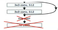
The input image is fed into a CNN, often called backbone, which is usually a pretrained network such as ResNet101. The classification (fully connected) layers from the backbone network are removed so as to use it as a feature extractor. This also makes the network fully convolutional, thus it can take any input size image.

The RPN uses a sliding window method to get relevant anchor boxes (the precalculated fixed sized bounding boxes having different sizes that are placed throughout the image that represent the approximate bbox predictions so as to save the time to search) from the feature maps.

It then does a binary classification that the anchor has object or not (into classes fg or bg), and bounding box regression to refine bounding boxes. The anchor is classified as positive label (fg class) if the anchor(s) has highest Intersection-over-Union (IoU) with the ground truth box, or, it has IoU overlap greater than 0.7 with the ground truth.

At each sliding window location, a number of proposals (max k) are predicted corresponding to anchor boxes. So the reg layer has 4k outputs encoding the coordinates of k boxes, and the cls layer outputs 2k scores that estimate probability of object or not object for each proposal.

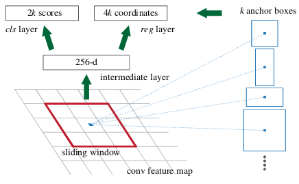
In Faster R-CNN, k=9 anchors representing 3 scales and 3 aspect ratios of anchor boxes are present at each sliding window position. Thus, for a convolutional feature map of a size W×H (typically∼2,400), there are WHk anchors in total.

Hence, at this stage, there are two losses i.e. bbox binary classification loss, \(L_{cls_1}\) and bbox regression loss, \(L_{bbox_1}\).

The top (positive) anchors output by the RPN, called proposals or Region of Interest (RoI) are fed to the next stage.

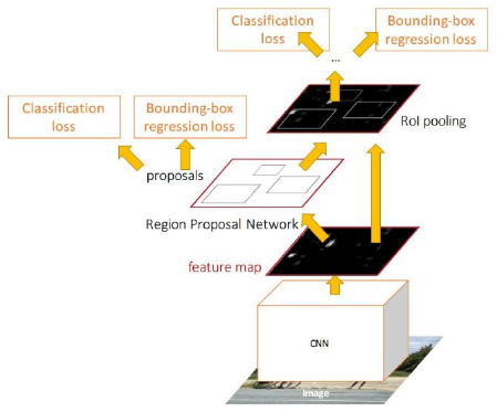
Stage II

The second stage is essentially Fast R-CNN, which using RoI pooling layer, extracts feature maps from each RoI, and performs classification and bounding box regression. The RoI pooling layer converts the section of feature map corresponding to each (variable sized) RoI into fixed size to be fed into a fully connected layer.

For example, say, for a 8x8 feature map, the RoI is 7x5 in the bottom left corner, and the RoI pooling layer outputs a fixed size 2x2 feature map. Then, the following operations would be performed:

• Divide the RoI into 2x2.
• Perform max-pooling i.e. take maximum value from each section.

The fc layer further performs softmax classification of objects into classes (e.g. car, person, bg), and the same bounding box regression to refine bounding boxes.

Thus, at the second stage as well, there are two losses i.e. object classification loss (into multiple classes), \(L_{cls_2}\), and bbox regression loss, \(L_{bbox_2}\).

Mask prediction

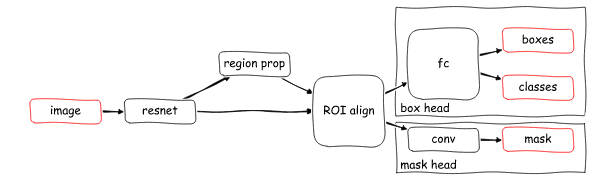
Mask R-CNN has the identical first stage, and in second stage, it also predicts binary mask in addition to class score and bbox. The mask branch takes positive RoI and predicts mask using a fully convolutional network (FCN).

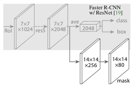
In simple terms, Mask R-CNN = Faster R-CNN + FCN

Finally, the loss function is

The \(L_{cls} (L_{cls_1} + L_{cls_2})\) is the classification loss, which tells how close the predictions are to the true class, and \(L_{bbox} (L_{bbox_1} + L_{bbox_2})\) is the bounding box loss, which tells how good the model is at localization, as discussed above. In addition, there is also \(L_{mask}\), loss for mask prediction, which is calculated by taking the binary cross-entropy between the predicted mask and the ground truth. This loss penalizes wrong per-pixel binary classifications (fg/bg w.r.t ground truth label).

Mask R-CNN encodes a binary mask per class for each of the RoIs, and the mask loss for a specific RoI is calculated based only on the mask corresponding to its true class, which prevents the mask loss from being affected by class predictions.

The mask branch has a \(Km^2\)-dimensional output for each RoI, which encodes K binary masks of resolution m×m, one for each of the K classes. To this we apply a per-pixel sigmoid, and define \(L_{mask}\) as the average binary cross-entropy loss.

In total, there are five losses as follows:

• rpn_class_loss, \(L_{cls_1}\): RPN (bbox) anchor binary classifier loss
• rpn_bbox_loss, \(L_{bbox_1}\): RPN bbox regression loss
• fastrcnn_class_loss, \(L_{cls_2}\): loss for the classifier head of Mask R-CNN
• fastrcnn_bbox_loss, \(L_{bbox_2}\): loss for Mask R-CNN bounding box refinement
• maskrcnn_mask_loss, \(L_{mask}\): mask binary cross-entropy loss for the mask head

Other improvements

Feature Pyramid Network

Mask R-CNN also utilizes a more effective backbone network architecture called Feature Pyramid Network (FPN) along with ResNet, which results in better performance in terms of both accuracy and speed.

Faster R-CNN with an FPN backbone extracts RoI features from different levels of the feature pyramid according to their scale, but otherwise the rest of the approach is similar to vanilla ResNet.

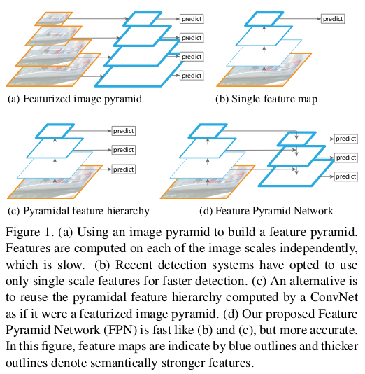
In order to detect object at different scales, various techniques have been proposed. One of them (c) utilizes the fact that deep CNN build a multi-scale representation of the feature maps. The features computed by various layers of the CNN acts as a feature pyramid. Here, you can use your model to detect objects at different levels of the pyramid thus allowing your model to detect object across a large range of scales e.g. the model can detect small objects at conv3 as it has higher spatial resolution thus allowing the model to extract better features for detection compared to detecting small objects at conv5, which has lower spatial resolution. But, an important thing to note here is that the quality of features at conv3 won’t be as good for classification as features at conv5.

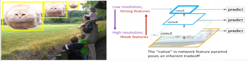
The above idea is fast as it utilizes the inherent working of CNN by using the features extracted at different conv layers for multi-scale detection, but compromises with the feature quality.

FPN uses the inherent multi-scale representation in the network as above, and solves the problem of weak features at later layers for multi-scale detection.

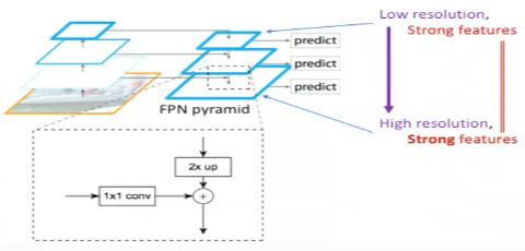
The forward pass of the CNN gives the feature maps at different conv layers i.e. builds the multi-level representation at different scales. In FPN, lateral connections are added at each level of the pyramid. The idea is to take top-down strong features (from conv5) and propagate them to the high resolution feature maps (to conv3) thus having strong features across all levels.

RoiAlign

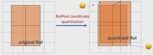
As discussed above, RoIPool layer extracts small feature maps from each RoI. The problem with RoIPool is quantization. If the RoI doesn’t perfectly align with the grid in feature map as shown, the quantization breaks pixel-to-pixel alignment. It isn’t much of a problem in object detection, but in case of predicting masks, which require finer spatial localization, it matters.

RoIAlign is an improvement over the RoIPool operation. What RoIAlign does is to smoothly transform features from the RoIs (which has different aspect sizes) into fixed size feature vectors without using quantization. It uses bilinear interpolation to do. A grid of sampling points are used within each bin of RoI, which are used to interpolate the features at its nearest neighbors as shown.

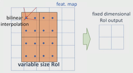
For example, in the above figure, you can’t apply the max-pooling directly due to the misalignment of RoI with the feature map grids, thus in case of RoIAlign, four points are sampled in each bin using bilinear interpolation from its nearest neighbors. Finally, the max value from these points is chosen to get the required 2x2 feature map.

Implementation

The following Mask R-CNN implementation is from facebookresearch/maskrcnn-benchmark in PyTorch.

Other famous implementations are:

• matterport’s Mask_RCNN in Keras and Tensorflow
• open-mmlab’s mmdetection in PyTorch
• facebookresearch’s Detectron in Caffe2, and Detectron2 in PyTorch

First, install it as follows.

# install dependencies
pip install ninja yacs cython matplotlib tqdm opencv-python

# install COCO API
git clone https://github.com/cocodataset/cocoapi.git
cd cocoapi/PythonAPI
python setup.py build_ext install
cd ../../

# install apex
rm -rf apex
git clone https://github.com/NVIDIA/apex.git
cd apex
git pull
# if no GPU available, try installing removing --cuda_ext
python setup.py install --cuda_ext --cpp_ext
cd ../

# install maskrcnn-benchmark 
git clone https://github.com/facebookresearch/maskrcnn-benchmark.git
cd maskrcnn-benchmark
# the following will install the lib with symbolic links, so that you can modify
# the files if you want and won't need to re-build it
python setup.py build develop

# download predictor.py, which contains necessary utility functions
wget https://raw.githubusercontent.com/facebookresearch/maskrcnn-benchmark/master/demo/predictor.py

# download configuration file
wget https://raw.githubusercontent.com/facebookresearch/maskrcnn-benchmark/master/configs/caffe2/e2e_mask_rcnn_R_50_FPN_1x_caffe2.yaml

Here, for inference, we’ll use Mask R-CNN model pretrained on MS COCO dataset.

import numpy as np
import matplotlib.pyplot as plt
import matplotlib.pylab as pylab
import requests
from io import BytesIO
from PIL import Image
from maskrcnn_benchmark.config import cfg
from predictor import COCODemo

config_file = "e2e_mask_rcnn_R_50_FPN_1x_caffe2.yaml"

# update the config options with the config file
cfg.merge_from_file(config_file)

# a helper class `COCODemo`, which loads a model from the config file, and performs pre-processing, model prediction and post-processing for us
coco_demo = COCODemo(
    cfg,
    min_image_size=800,
    confidence_threshold=0.7,
)

pil_image = Image.open('cats.jpg').convert("RGB")
# convert to BGR format
image = np.array(pil_image)[:, :, [2, 1, 0]]

# compute predictions
predictions = coco_demo.run_on_opencv_image(image)

# plot
f, ax = plt.subplots(1, 2, figsize=(15, 4))
ax[0].set_title('input image')
ax[0].axis('off')
ax[0].imshow(pil_image)
ax[1].set_title('segmented output')
ax[1].axis('off')
ax[1].imshow(predictions[:, :, [2, 1, 0]])
plt.savefig("segmented_output.png", bbox_inches='tight')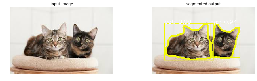

Notice that, here, both the instances of cats are segmented separately, unlike semantic segmentation.

Other Instance segmentation models

MS R-CNN (Mask Scoring R-CNN)

In Mask R-CNN, the instance classification score is used as the mask quality score. However, it’s possible that due to certain factors such as background clutter, occlusion, etc. the classification score is high, but the mask quality (IoU b/w instance mask and ground truth) is low. MS R-CNN uses a network that learns the quality of mask. The mask score is reevaluated by multiplying the predicted MaskIoU and classification score.

Within the Mask R-CNN framework, we implement a MaskIoU prediction network named MaskIoU head. It takes both the output of themask head and RoI feature as input, and is trained using a simple regression loss.

i.e. MS R-CNN = Mask R-CNN + MaskIoU head module

YOLACT (You Only Look At CoefficienTs)

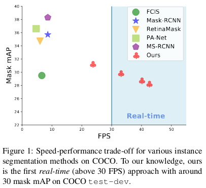
YOLACT is the current fastest instance segmentation method. It can achieve real-time instance segmentation results i.e. 30fps.

It breaks the instance segmentation process into two parts i.e. it generates a set of prototype masks in parallel with predicting per-instance mask coefficients. Then the prototypes are linearly combined with the mask coefficients to produce the instance masks.

References & Further Readings:

1. Mask R-CNN paper
2. Faster R-CNN paper
3. FPN paper
4. MS R-CNN paper
5. YOLACT paper
6. Mask R-CNN presented by Jiageng Zhang, Jingyao Zhan, Yunhan Ma
7. Tutorial: Deep Learning for Objects and Scenes - Part 1 - CVPR’17
8. CS231n: Convolutional Neural Networks for Visual Recognition (image source)
9. Mask R-CNN image source
10. RoIPool image source