Object detection deals with the detection of object instances in an image. There are a number of methods to accomplish it. The following post summarizes few important object detection methods.
Classification and Localization
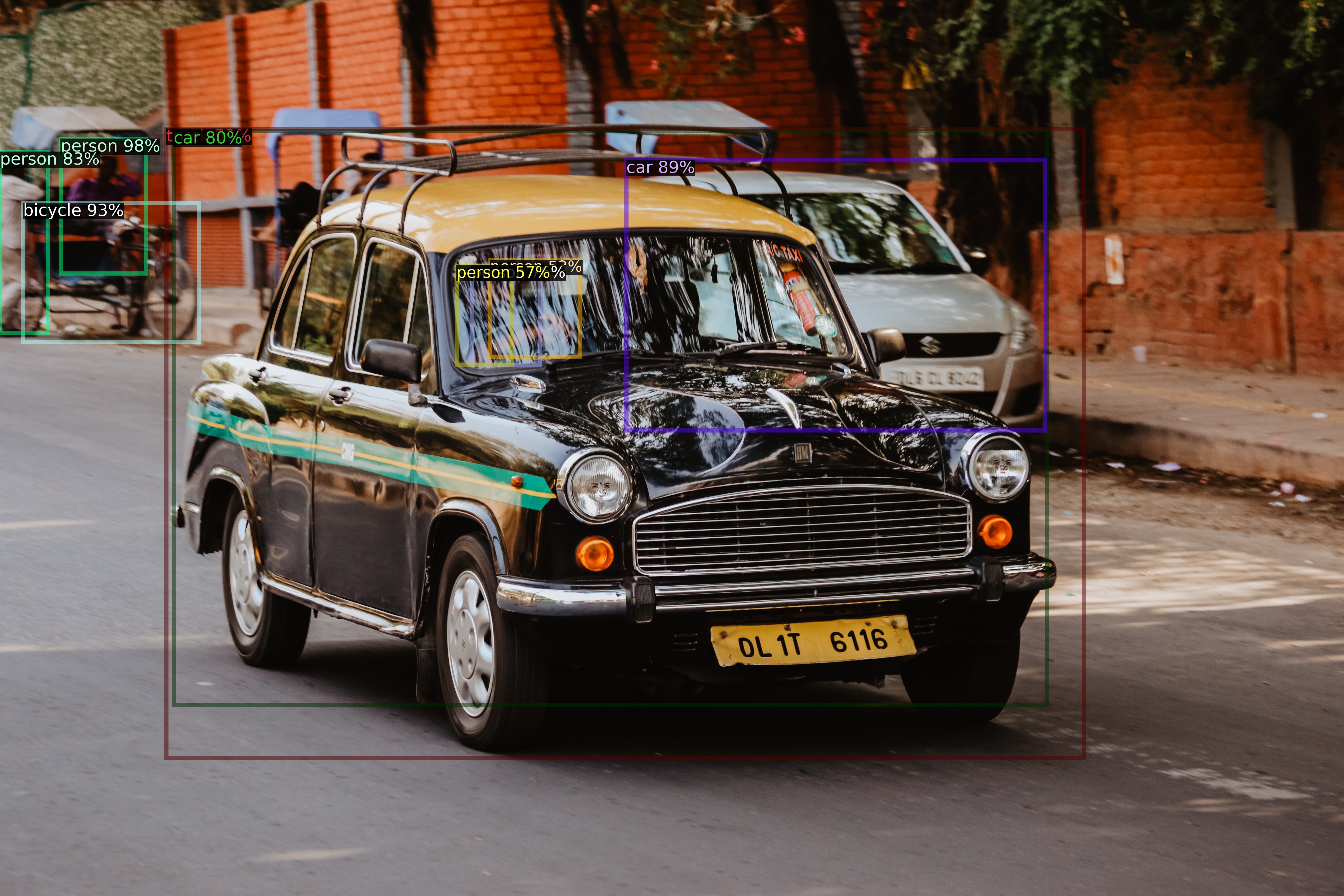
This method treats object detection as a regression problem. Given an object in an image, localization deals with by drawing a bounding box around the object by finding its location in the image. The classification refers to categorizing the object into the class labels such as cat, dog, etc. The object detection problem refers to the same scenario in multi-object context i.e. Given a number of objects in an image, object detection is defined as the classification as well as localization of all the objects in the image.
With the help of a fully connected layer, fc, a model can be used to classify an object into categories such as cat, dog, …, and background (if none of the object detected). In order to do localization, the model can be modified to give the bounding box coordinates, \(b_x, b_y, b_h, b_w\) representing the x and y coordinate of the center of object, and height and width respectively. This model can be trained in order to perform object detection such that the target label y can be defined as
where \(p_c\) is the probability of the object (0 if background, no object), and \(c_1, c_2, ..., c_m\) are the class probabilities.
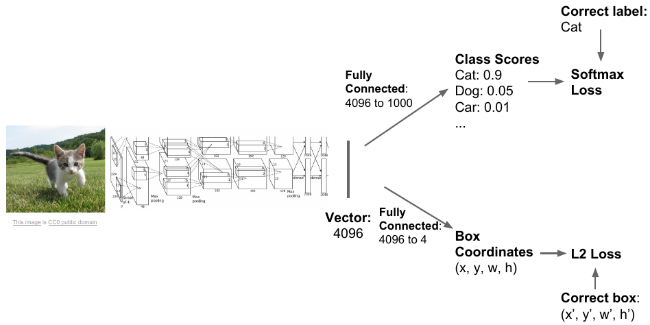
The loss may consists of softmax loss for classification and L2 regression loss for bounding box. The problem with this approach is that an image may contain different number of objects thus each image need different number of outputs, which creates a problem.
Sliding window
This method treats object detection as a classification problem. The sliding window deals with sliding the window through the image and passing the cropped image to a convolutional neural network and classifying it as object or background.
The problem with this approach is that it’s needed to apply CNN to a huge number of windows of diverse scale and aspect ratio.
Region proposals
The region proposal methods deals with using selective search to propose regions (boxes) that likely contain objects thus avoiding the computationally expensive method of appplying CNN to every possible window in the image.
The various region based methods i.e. region-proposals are:
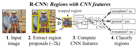
- R-CNN: First, the Region of Interest (ROI) is suggested by a region proposal method. These regions are then fed into CNN and support vector machines is used to classify them.
- Fast R-CNN: Instead of passing each region through CNN, in Fast R-CNN the entire image is passed once generating convolutional feature maps, using which the regions are proposed. The ROI pooling layer is then used to convert these regions into a fixed size, finally feeding it into a fully connected network.
- Faster R-CNN: Unlike Fast R-CNN which uses selective search for ROI, Faster R-CNN uses Region Proposal Network (RPN) to predict proposals from features.
- Mask R-CNN: It extends Faster R-CNN. Mask R-CNN is used for instance segmentation which not only does object detection but also predicts object masks.
Read more about how Faster R-CNN and Mask R-CNN work in the instance segmentation post.
Detection without proposals
There are other object detection methods that use detection without proposals. The following methods are faster though not as good in terms of accuracy compared to R-CNN family.
YOLO (You Only Look Once)
What YOLO does is to divide the input image into a grid, and apply the classification and localization to each of these grids. Here, each grid predicts one object defined by the same label y discussed above. An object is said to belong to a particular grid cell if its center lies in it. Hence, for each of the SxS grid cells, there is a 5+C dimension y label, where C is the number of classes.
But in YOLO, each grid cell predicts a number of bboxes (not one), B, for the single object it detects. Hence, the YOLO prediction is of the form SxSx(B*5+C). Suppose, an image is divided into a grid of 3x3, and B=4, and number of class labels is 2, then the YOLO prediction volume will be of shape (3, 3, 22).
IoU (Intersection over Union)
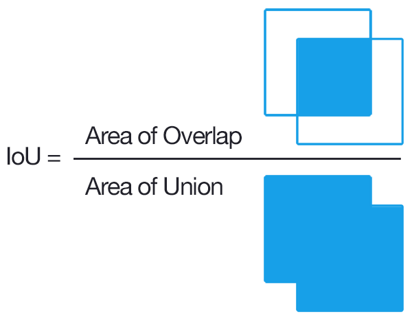
To decide whether a prediction is correct w.r.t to an object or not, IoU or Jaccard Index is used. It is defines as the intersection b/w the predicted bbox and actual bbox divided by their union. A prediction is considered to be True Positive if IoU > threshold.
Non-max suppression
It might happen that more than one grid cell may predict the same object such that there are multiple bbox detections for the same object. The NMS (Non-max suppression) enables to get a single detection per object. This is how it works.
- Discard all bbox where \(p_c < \text{threshold}\).
- For each remaining bbox:
2.1 Pick bbox with the highest \(p_c\), and output it as a prediction.
2.2 Discard any remaining bbox with high overlap,IoU > 0.5, with the output in the previous step.
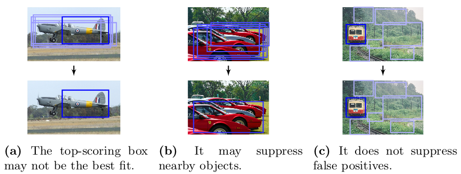
Note that this greedy approach suffers from certain problems such as the assumption that the best scoring \(p_c\) is the best fit for the object.
Anchors
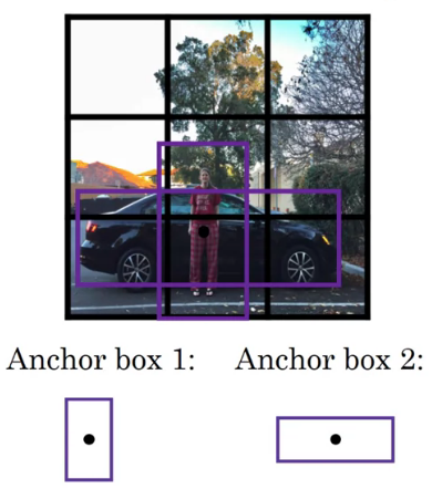
Since we discussed that each grid cell may predict only a single object, it won’t be able to detect two different objects such as car and person, even if their centers lie in that grid cell thus ignoring one of the object. This is not what we want. The anchor boxes or priors allow multiple detections per grid cell. These are precalculated fixed bbox representing the approximate bbox prediction. Now, each object is assigned to a grid cell that contains its midpoint, and anchor box of the grid cell with hightest IoU.
Hence, the y label now has multiple predictions w.r.t. anchor box.
Not only anchor boxes allows multiple detections per grid cell, but they also allow the model to learn quickly by providing it the starting coordinates to finetune.
SSD (Single Shot Multibox Detector)
The SSD also performs the localization and classification in a single forward pass similar to YOLO. The multibox is the technique that treats the bbox prediction as a regression problem by taking anchors (priors) as the starting point for bbox prediction and regressing them to the ground truth bbox’s coordinates.
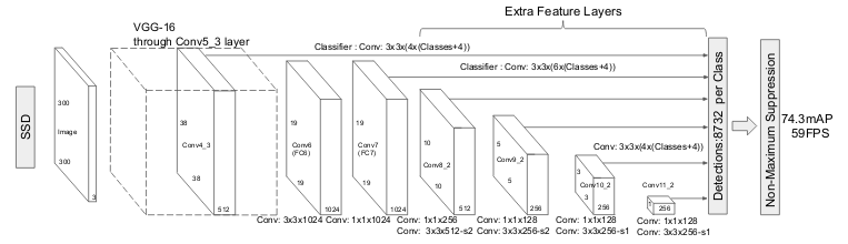
SSD takes the VGG network, called base network, and converts its fc layers to conv layers, and further add more convolutional layers, called auxiliary convolutions, to create a powerful feature extractor. It allows predictions at different scales from the feature maps of different scales produced by these layers as they decrease in size progressively. It also applies the NMS to produce the final detections.
The multibox loss is weighted sum of localization loss, \(L_{\text{loc}}\), for bbox, and classification confidence loss, \(L_{\text{conf}}\) for object classes.
\[L = L_{\text{loc}} + \alpha * L_{\text{conf}}\]where the localization loss is the averaged smooth L1 loss b/w the predicted bbox coordinates and its ground truths.
\[L_{\text{loc}} = \frac{1}{n_{\text{postives}}}\sum_{positives}{\text{smooth $L_1$ loss}}\]Hard Negative Mining
Most of the bbox predictions would be negative as only a handful of predictions would contain an object. It’d result in the imbalance of positive to negative examples, which is not good for training the model.
The solution, called Hard Negative Mining, is to limit the number of negatives and only use those predictions where the model find it hardest to predict the object.
Instead of using all the negative examples, we sort them using the highest confidence loss for each default box and pick the top ones so that the ratio between the negatives and positives is at most 3:1. We found that this leads to faster optimization and a more stable training.
Thus, the confidence loss is the sum of cross entropy losses in positive and negative matches.
\[L_{\text{conf}} = \frac{1}{n_{\text{postives}}}\left(\sum_{positives}{\text{cross-entropy loss}} + \sum_{\text{hard negatives}}{\text{cross-entropy loss}}\right)\]References & Further Readings:

Comments