Attention is the technique through which the model focuses itself on a certain region of the image or on certain words in a sentence just like the same way the humans do. For example, when looking at an image, humans shifts their attention to different parts of the image one at a time rather than focusing on all parts in equal amount at the same time.

Encoder-Decoder architecture

A Recurrent Neural Network (RNN) can be used to map a varied-length input sequence to the varied-length output sequence e.g. machine translation. The simplest sequence-to-sequence architecture that makes it possible consists of two models, Encoder, and Decoder. In Encoder-Decoder architecture, the idea is to learn a fixed-size context vector that contains the essential information of the inputs.

• The Encoder processes the input sequence \((x_1, x_2, x_3, ..., x_n)\) and gives a context vector, C that summarizes the input sequence.
• The Decoder uses C to generate the output sequence \((y_1, y_2, y_3, ..., y_m)\), where n and m may not be equal.

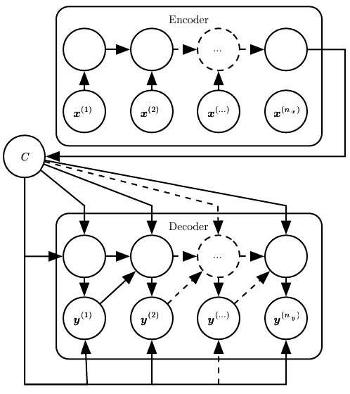
The final hidden state of the hidden state of encoder RNN is used to compute C, which is further provided as an input to the decoder.

The problem with encoder-decoder approach is that all the input information needs to be compressed in a fixed length context vector, C. It makes it difficult for the network to cope up with large amount of input information (e.g. in text, large sentences) and produce good results with only that context vector. With attention mechanism, the encoder RNN instead of producing a single context vector to summarize the input image or sequence, produces a grid of vectors. That is, attention makes C a variable-length sequence rather than a fixed-size vector.

Every step in the decoder (only) requires calculation of attention vector in seq2seq model. The Attention decoder uses a scoring function to score each hidden state. These scores when fed into a softmax function gives the weight of each vector in the attention vector. Now, these weights are multiplied by corresponding hidden state vector, whose sum gives the attention context vector. The decoder at each step looks at input sequence as well as attention context vector, which focuses its attention at appropriate place in input sequence, and produces the hidden state.

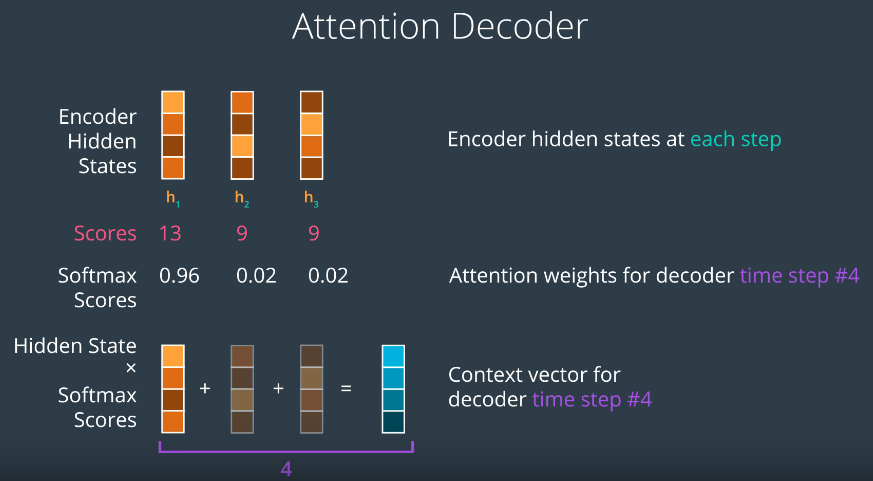
The important part is that each decoder output \(y_t\) now depends on a weighted combination of all the input states, not just the last state.

The decoder has hidden state \(s_t=f(s_{t−1},y_{t−1},c_t)\) for the output word at position t, where t=1,…,m, where the context vector \(c_t\) is a sum of hidden states of the input sequence, weighted by alignment scores

The alignment model assigns a score \(α_{t,i}\) to the pair of input at position i and output at position t, \((y_t,x_i)\), based on how well they match. The set of scores \(\{\alpha_{t, i}\}\) are weights defining how much of each source hidden state should be considered for each output.

Attention Types

Attention mechanisms differ in how they compute the alignment score between the query (decoder hidden state) and keys (encoder hidden states).

Dot-product (Scaled Dot-Product Attention)

The simplest method. Computes the attention score as the dot product of the query and key vectors, scaled by the square root of the key dimension to stabilize gradients:

This is the attention mechanism used in the Transformer architecture, where it’s computed efficiently in matrix form:

Bilinear Function (Luong Attention)

Introduces a learnable weight matrix \(W_a\) to capture more complex interactions between query and key vectors:

Multi-Layer Perceptron (Bahdanau / Additive Attention)

Uses a feedforward network with a \(\tanh\) activation to compute attention scores, allowing for non-linear interactions:

This was the original attention mechanism proposed by Bahdanau et al. for neural machine translation.

Transformer Architecture

The Transformer extends the attention mechanism into a full encoder-decoder architecture without recurrence. The encoder consists of N=6 identical layers, each with:

1. Multi-head Self-Attention: Allows each position to attend to all positions in the input sequence. The mechanism runs multiple attention heads in parallel with different learned projections of Q, K, V, capturing different aspects and dependencies.
2. Position-wise Feedforward Networks: Applied independently to each position. Includes a residual connection around each sub-layer, followed by layer normalization.

The decoder also has N=6 identical layers, each with three sub-layers:

1. Masked Multi-head Self-Attention: Prevents positions from attending to subsequent positions (preserving auto-regressive property). Future positions are masked (set to \(-\infty\)) before the softmax step.
2. Encoder-Decoder Attention (Cross-Attention): Queries come from the decoder, keys and values from the encoder output, allowing the decoder to focus on relevant parts of the input.
3. Position-wise Feedforward Networks: Same as the encoder.

Self-Attention Walkthrough

For a sentence like “The cat sat on the mat.”, self-attention for the word “sat” works as follows:

1. Create Query, Key, Value vectors for each word by multiplying embeddings with learned weight matrices \(W_q, W_k, W_v\).
2. Compute attention scores by taking the dot product of “sat”’s query with every word’s key. “sat” will have the highest score with itself (0.82), but also attends to “the” (0.31), “cat” (0.61), “on” (0.52), etc.
3. Scale scores (divide by \(\sqrt{d_k}\)), apply softmax to get attention weights.
4. Multiply each value vector by its attention weight and sum, producing a context-aware representation for “sat”.

Positional Encoding

Since Transformers process the entire sequence in parallel (no recurrence), positional information is injected via positional encodings. The original Transformer uses sinusoidal functions:

\(PE_{(pos, 2i)} = \sin(pos / 10000^{2i/d_{model}})\) \(PE_{(pos, 2i+1)} = \cos(pos / 10000^{2i/d_{model}})\)

Unlike learned embeddings, sinusoidal encodings can extrapolate to sequence lengths unseen during training. The cyclic nature of sine/cosine functions naturally mirrors the intuition that nearby words tend to have stronger relationships than distant ones.

Transformers vs RNNs/LSTMs

• Parallelization: Self-attention allows parallel computation across the entire input sequence.
• Long-range dependencies: Self-attention provides direct connections between any two positions, enabling gradient flow across longer distances compared to the compressed context vector of RNNs.
• Vanishing gradients: The residual connections in Transformers mitigate the vanishing gradient problem common in RNNs.

Further Readings:

1. Attention and Memory in Deep Learning and NLP
2. How Does Attention Work in Encoder-Decoder Recurrent Neural Networks
3. Attention? Attention!
4. PyTorch Deep Learning Nanodegree - Udacity (also image source)