Backpropagation Through Time
Friday, February 22, 20193 mins read
In the earlier post The gradient problem in RNN, you came to know that RNNs have exploding and vanishing gradient problems. This post discusses how exactly the gradients are calculated in RNNs. Let’s take a deep dive into the mathematics of RNNs.
The equation
\[s_t = f_W(s_{t-1}, x_t)\]defines the RNN structure. Here, \(s_t\) is the state vector at time t. It can be written as
Here, \(\phi\) is the activation function say \(tanh\). The output vector can be written as
\[y_t = W_y s_t\]The loss function or simply the output error at time t can be written as


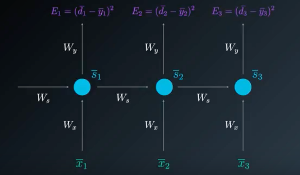
The unrolled representation of RNN is shown

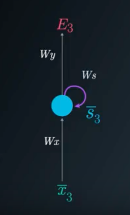
Here, \(W_x\), \(W_y\) and \(W_s\) represent the weight matrices connecting the inputs to the state layer, connecting the state to the output and connecting the state from the previous timestep to the state in the following timestep respectively.
The backpropagation algorithm applied to this unrolled (unfolded) graph of RNN is called backpropagation through time (BPTT). RNN takes into account its history i.e. the previous states as evident from its equation. The current state depends on the input as well as the previous states. Thus to update the weights, the gradient of loss function at particular time step t depends not only on the input but also on the gradients of previous states at all the previous time steps. The total loss for a given sequence of input values paired with a sequence of output values would be the sum of the losses over all the time steps.
Gradient calculations to update \(W_y\)
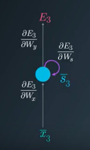
Using chain rule, the gradient of loss function w.r.t. \(W_y\) at 3rd timestep
\[\frac{\partial E_3}{\partial W_y} = \frac{\partial E_3}{\partial y_3} \frac{\partial y_3}{\partial W_y}\]Gradient calculations to update \(W_s\)
The partial derivate of loss function w.r.t. \(W_s\) depends on state \(s_3\), which depends on \(s_2\), which further depends on its predecessor \(s_1\), the first state. Hence, all these gradients are to be accumulated to update \(W_s\) i.e.
\[\frac{\partial E_3}{\partial W_s} = \text{gradient from} s_3 + \text{gradient from} s_2 + \text{gradient from} s_1\] \[\frac{\partial E_3}{\partial W_s} = \frac{\partial E_3}{\partial y_3} \frac{\partial y_3}{\partial s_3} \frac{\partial s_3}{\partial W_s} + \frac{\partial E_3}{\partial y_3} \frac{\partial y_3}{\partial s_3} \frac{\partial s_3}{\partial s_2} \frac{\partial s_2}{\partial W_s} + \frac{\partial E_3}{\partial y_3} \frac{\partial y_3}{\partial s_3} \frac{\partial s_3}{\partial s_2} \frac{\partial s_2}{\partial s_1} \frac{\partial s_1}{\partial W_s}\]In the same way, the gradient of loss w.r.t. \(W_x\) can be calculated. The general formula for gradient calculation is
\[\frac{\partial y}{\partial W} = \sum_{i=t+1}^{t+N} \frac{\partial y}{\partial s_{t+N}} \frac{\partial s_{t+N}}{\partial s_i} \frac{\partial s_i}{\partial W}\]Truncated Backpropagation through time (TBPTT)
The problem with BPTT is that the update in weights require forward through entire sequence to compute loss, then backward through entire sequence to compute gradient. The slight variant of this algorithm called Truncated Backpropagation through time (TBPTT), where forward and backward pass are run through chunks of sequences instead of the whole sequence. It’s similar to using mini-batches in gradient descent i.e. the gradients are calculated for each step, but the weights get updated in batches periodically (as opposed to once every inputs sample). This helps reduce the complexity of the training process and helps remove noise from the weight updates. But the problem with TBPTT is that the network can’t learn long dependencies as in BPTT because of limit on flow of gradient due to truncation.
Note that backpropagating for large number of steps leads to the gradient problems.
References: