Natural Language Processing deals with the task of making computer understand the human language. The computer understands only 0s and 1s. A language consists of words. So, the first task is to convert word into a combination of 0s and 1s. This is easy. But, a word is nothing without its meaning. Hence, the task we need to solve is to represent the meaning of a word.

Representing words as discrete symbols

One solution to this problem is to use one-hot vector. For example, in the sentence, “I love machine learning”, the word machine can be represented as [0, 0, 1, 0] where 1 corresponds to machine. In the same way, we can represent other words such as learning, [0, 0, 0, 1].

The problem with this approach is that the combination of words has no meaning i.e. to match “machine learning” in a given document. we have got two separate vectors of machine and learning, which unfortunately are orthogonal. Thus, such a search will not yield any result. That is, there is no notion of similarity for one-hot vectors.

Representing words by their contexts

The core idea in this approach is that the words are represented by the context they have i.e. a word’s meaning is given by the words that frequently surrounds it.

word2vec¹ is a model for learning word vectors.

While talking about word2vec, we focus on two model variants:

• Skip-grams (SG): Predict context words (position independent) given center word
• Continuous Bag of Words (CBOW): Predict center word from (bag of) context words

Every word in vocabulary is represented by a vector. In Skip-gram model, we use the similarity of word vectors to calculate the probability of a word being context word. The word vectors are adjusted to maximize this probability.

The below figure demonstrates example windows and process for computing \(P(w_{t+2} \mid w_t)\).

We can implement word2vec model in python:

from genism.model import Word2Vec

Word embeddings

The word vectors, discussed above, are called embeddings (encoding words to numbers) and are learnt in the same way as other hyperparameters in a neural network.

word embeddings are a representation of the semantics of a word, efficiently encoding semantic information that might be relevant to the task at hand.

While designing neural networks, an embedding layer is used. The word2vec model such as CBOW is used to learn word embeddings. Instead of learning the embeddings every time in a network, these pretrained embeddings (already learnt using word2vec) can be used to initialize the embeddings of the network.

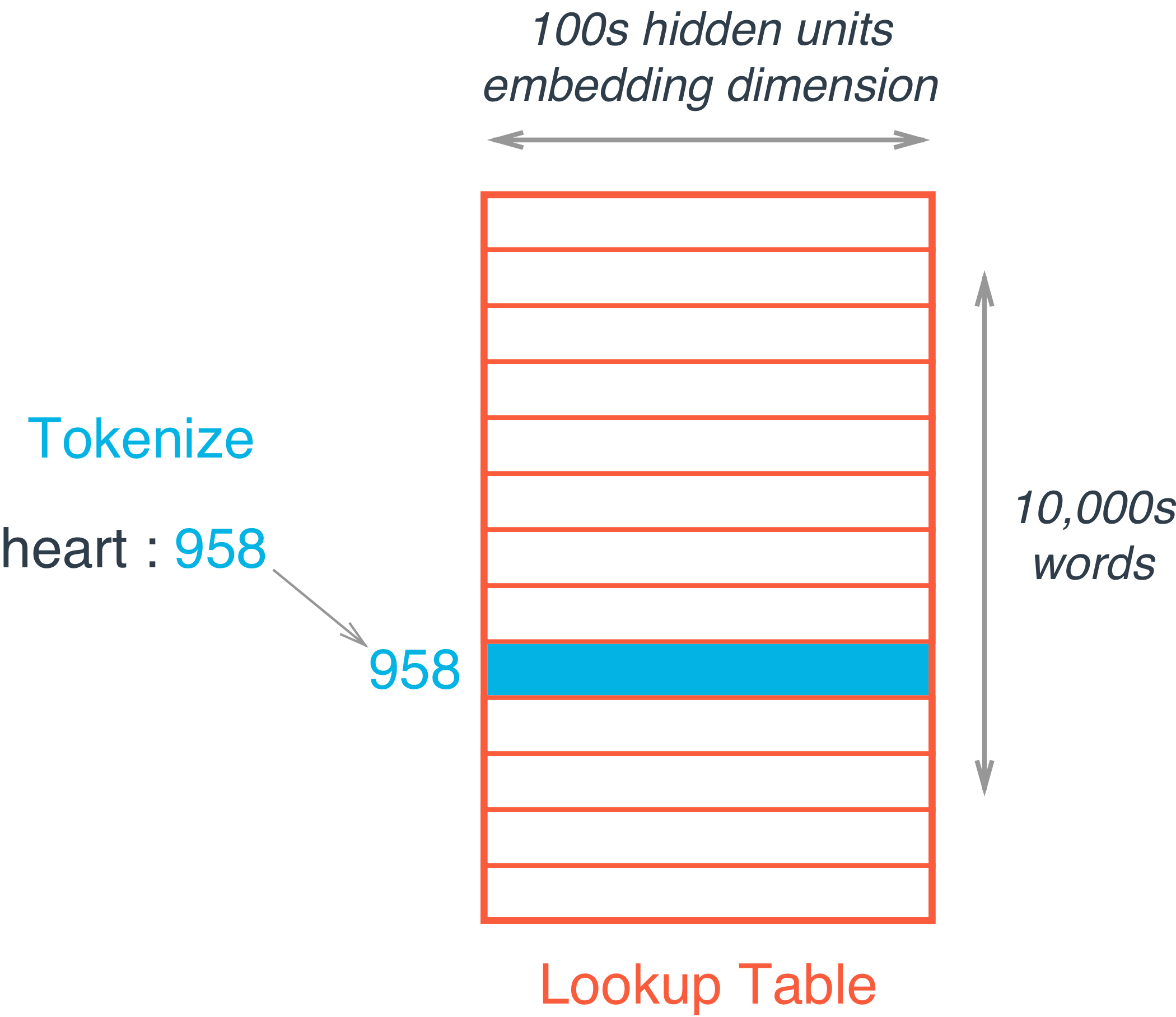
This embedding layer is just like a hidden layer, which behaves as a lookup table i.e. instead of doing matrix multiplication, the embedding of a particular word can be extracted from the weight matrix of embeddings using an index. For example “heart” is encoded as 958. Then to get embedding for “heart”, you just take the 958th row of the embedding matrix. It’s possible because the multiplication of a one-hot encoded vector with a matrix returns the row of the matrix corresponding the index of the “on” input unit.

The embeddings are stored as a \(\|V\| \times D\) matrix, where V is our vocabulary, and D is the dimensionality of the embeddings, such that the word assigned index i has its embedding stored in the i‘th row of the matrix. For hidden dimensions (for most of the problems), D, any number between 200-500 should work. It’s kind of a hyperparameter. There’s no precise number.

The embedding vector dimension should be the 4th root of the number of categories i.e. 4th root of the vocab size. You can choose it as a rule of thumb. — Google Developer’s blog²

Bag of Words

The Bag of Words model treats each document (text units) as a bag (collection) of words. A set of documents is called a corpus. First, collect all unique words from your corpus to form vocabulary and arrange them into a matrix of vectors by number of occurrences of each word. This matrix is called Document-Term-Matrix where each document is a row and unique words are columns. Each element is called a term frequency, which denotes how many times that term occur in the corresponding document. To calculate the similarity of words, the term-frequency can be compared using cosine-similarity, given by dot product of two vectors and divided by their magnitudes.

References:
1: word2vec: Efficient Estimation of Word Representations in Vector Space ↩
2: Google Developer’s blog ↩
3: An Intuitive Understanding of Word Embeddings: From Count Vectors to Word2Vec