Much as Convolutional Neural Networks are used to deal with images, the Recurrent Neural Networks are used to process sequential data. The key idea in recurrent neural networks is parameter sharing across different parts of the model i.e. a RNN shares same weights across several time steps. As feedforward neural network can model any function, a recurrent neural network can model any function involving recurrence.

RNN

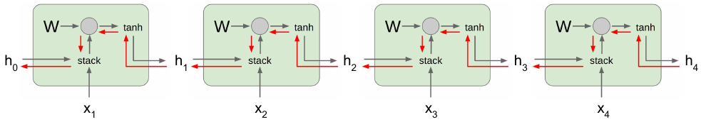
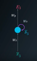
The vanilla Recurrent Neural Network (RNN) has the following structure:

Here, the same function and same set of parameters are used at every time step. The \(h_t\) denotes the state, which is a kind of summary of past sequence of inputs \((x_t, x_{t-1}, x_{t-2}, ..., x_1)\) upto \(t\) mapped to fixed length vector \(h_t\).

But, the gradient flow in RNNs often lead to the following problems:

• Exploding gradients
• Vanishing gradients

The gradient computation involves recurrent multiplication of \(W\). This multiplying by \(W\) to each cell has a bad effect. Think like this: If you a scalar (number) and you multiply gradients by it over and over again for say 100 times, if that number > 1, it’ll explode the gradient and if < 1, it’ll vanish towards 0.

In the backpropagation process, we adjust our weight matrices with the use of a gradient. In the process, gradients are calculated by continuous multiplications of derivatives. The value of these derivatives may be so small, that these continuous multiplications may cause the gradient to practically “vanish”.

The problem of exploding gradients can be solved by gradient clipping i.e. if gradient is larger than the threshold, scale it by dividing. LSTM solves the problem of vanishing gradients.

LSTM

A Long Short Term Memory (LSTM) utilizes four gates that perform a specific function.

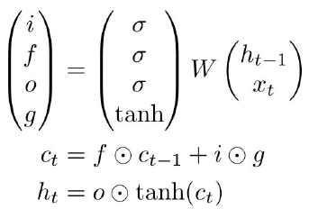
• Input gate (\(i\)): controls what to write to the LSTM cell
• Forget gate (\(f\)): controls whether to erase the cell
• Output gate (\(o\)): controls how much to reveal cell
• The fourth gate (\(g\)) controls how much to write to the cell

Inside the cell state, we can either remember or forget our previous state, and we can either increment or decrement each element of that cell state by up to 1 in each time step. These cell states can be interpreted as counters (counting by 1 or -1 at each time step). We want to squash that counter value in [0, 1] range using tanh. Then, we use our updated cell state to calculate our hidden state, which we’ll reveal to outside world.

The first step in our LSTM is to decide what information we’re going to throw away from the cell state. This decision is made by a sigmoid layer called the “forget gate layer.” It looks at \(h_{t-1}\) and \(x_t\), and outputs a number between 0 and 1 for each number in the cell state \(c_{t−1}\). A 1 represents “completely keep this” while a 0 represents “completely get rid of this.”

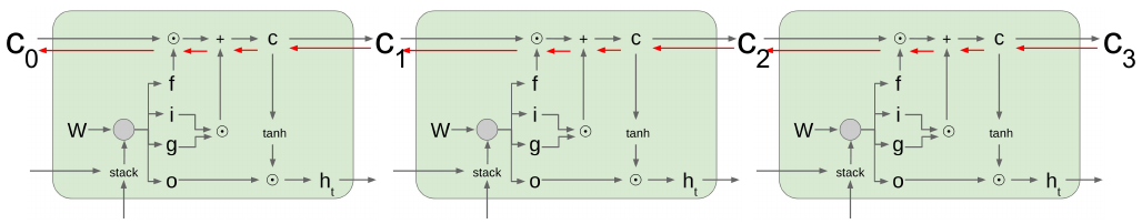
The next step is to decide what new information we’re going to store in the cell state. This has two parts. First, a sigmoid layer called the “input gate layer” decides which values we’ll update. Next, a tanh layer creates a vector of new candidate values, \(c_t\), that could be added to the state. In the next step, we’ll combine these two to create an update to the state.

Finally, we need to decide what we’re going to output. This output will be based on our cell state, but will be a filtered version. First, we run a sigmoid layer which decides what parts of the cell state we’re going to output. Then, we put the cell state through tanh (to push the values to be between −1 and 1) and multiply it by the output of the sigmoid gate, so that we only output the parts we decided to.

In LSTM, the backpropagation only involves element-wise multiplication by \(f\), and no matrix multiplication by \(W\) i.e. the cell state gradient is multiplied only by the forget gate element-wise (better than full matrix multiplication). Also, in vanilla RNN, we’re multiplying by same \(W\) over and over again leading to exploding or vanishing gradient problems. But, here this forget gate will vary at each time-step (e.g. values sometimes > 1 or < 1) thus avoiding these problems.

References:

1. CS231n: Convolutional Neural Networks for Visual Recognition (also image source)