Suppose you’ve an image, consisting of cats. You want to classify every pixel of the image as cat or background. This process is called semantic segmentation.

One of the ways to do so is to use a Fully Convolutional Network (FCN) i.e. you stack a bunch of convolutional layers in a encoder-decoder fashion. The encoder downsamples the image using strided convolution giving a compressed feature representation of the image, and the decoder upsamples the image using methods like transpose convolution to give the segmented output (Read more about downsampling and upsampling).

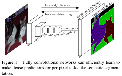
The fully connected (fc) layers of a convolutional neural network requires a fixed size input. Thus, if your model is trained on an image size of 224x224, the input image of size 227x227 will throw an error. The solution, as adapted in FCN, is to replace fc layers with 1x1 conv layers. Thus, FCN can perform semantic segmentation for any input size image.

In FCN, the skip connections from the earlier layers are also utilized to reconstruct accurate segmentation boundaries by learning back relevant features, which are lost during downsampling.

Semantic segmentation faces an inherent tension between semantics and location: global information resolves what while local information resolves where… Combining fine layers and coarse layers (by using skip connections) lets the model make local predictions that respect global structure.

U-Net

The U-Net build upon the concept of FCN. Its architecture, similar to the above encoder-decoder architecture, can be divided into three parts:

• The contracting or downsampling path consists of 4 blocks where each block applies two 3x3 convolution (+batch norm) followed by 2x2 max-pooling. The number of features maps are doubled at each pooling layer (after each block) as 64 -> 128 -> 256 and so on.
• The horizontal bottleneck consists of two 3x3 convolution followed by 2x2 up-convolution.
• The expanding or upsampling path, complimentary to the contracting path, also consists of 4 blocks, where each block consists of two 3x3 conv followed by 2x2 upsampling (transpose convolution). The number of features maps here are halved after every block.

The pretrained models such as resnet18 can be used as the left part of the model.

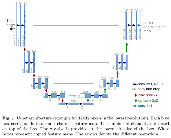
U-Net also has skip connections in order to localize, as shown in white. The upsampled output is concatenated with the corresponding cropped (cropped due to the loss of border pixels in every convolution) feature maps from the contracting path (the features learned during downsampling are used during upsampling).

Finally, the resultant output passes through 3x3 conv layer to provide the segmented output, where number of feature maps is equal to number segments desired.

DeepLab

DeepLab is a state-of-the-art semantic segmentation model having encoder-decoder architecture. The encoder consisting of pretrained CNN model is used to get encoded feature maps of the input image, and the decoder reconstructs output, from the essential information extracted by encoder, using upsampling.

To understand the DeepLab architecture, let’s go through its fundamental building blocks one by one.

Spatial Pyramid Pooling

In order to deal with the different input image sizes, fc layers can be replaced by 1x1 conv layers as in case of FCN. But we want our model to be robust to different size of input images. The solution to deal with variable sized images is to train the model on various scales of the input image to capture multi-scale contextual information.

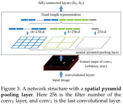
Usually, a single pooling layer is used between the last conv layer and fc layer. DeepLab, instead, utilizes a technique of using multiple pooling layer called Spatial Pyramid Pooling (SPP) to deal with multi-scale images. SPP divides the feature maps from the last conv layer into a fixed number of spatial bins having size proportional to the image size. Each bin gives a different scaled image as shown in the figure. The output of the SPP is a fixed size vector FxB, where F is the number of filters (feature maps) in the last conv layer, and B is the fixed number of bins. The different output vectors (16x256-d, 4x256-d, 1x256-d) are concatenated to form a fixed (4x4+2x2+1)x256=5376 dimension vector, which is fed into the fc layer.

There is a drawback to SPP that it leads to an increase in the computational complexity of the model, the solution to which is atrous convolution.

Dilated or atrous convolutions

Unlike the normal convolution, dilation or atrous convolution has one more parameter called dilation or atrous rate, r, which defines the spacing between the values in a kernel. The dilation rate of 1 corresponds to the normal convolution. DeepLab uses atrous rates of 6, 12 and 18.

The benefit of this type of convolution is that it enlarges field of view of filters to incorporate larger context without increasing the number of parameters.

Deeplab uses atrous convolution with SPP called Atrous Spatial Pyramid Pooling (ASPP). In DeepLabv3+, depthwise separable convolutions are applied to both ASPP and decoder modules.

Depthwise separable convolutions

Suppose you’ve an input RGB image of size 12x12x3, the normal convolution operation using 5x5x3 filter without padding and stride of 1 gives the output of size 8x8x1. In order to increase the number of channels (e.g. to get output of 8x8x256), you’ll have to use 256 filters to create 256 8x8x1 outputs and stack them together to get 8x8x256 output i.e. 12x12x3 — (5x5x3x256) —> 12x12x256. This whole operations costs 256x5x5x3x8x8=1,228,800 multiplications.

The depthwise separable convolution dissolves the above into two steps:

• In depthwise convolution, the convolution operation is perfomed separately for each channel using three 5x5x1 filter, stacking whose outputs gives 8x8x3 image.
• The pointwise convolution is used to increase the depth, number of channels, by taking convolution of 256 1x1x3 filters with the 8x8x3 image, where each filter gives 8x8x1 image which are stacked together to get 8x8x256 desired output image.

The process can be described as 12x12x3 — (5x5x1x1) —> (1x1x3x256) —> 12x12x256. This whole operation took 3x5x5x8x8 + 256x1x1x3x8x8 = 53,952 multiplication, which is far less compared to that of normal convolution.

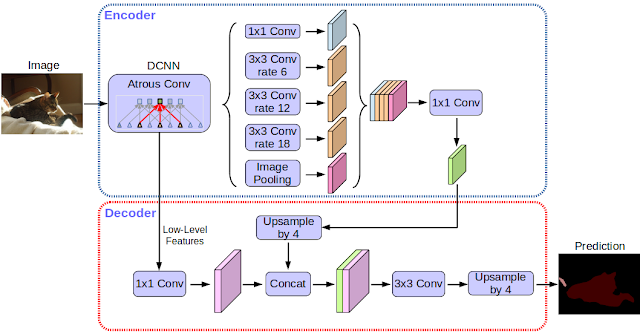
DeepLabv3+ uses xception (pointwise conv is followed by depthwise conv) as the feature extractor in the encoder portion. The depthwise separable convolutions are applied in place of max-pooling. The encoder uses output stride of 16, while in decoder, the encoded features by the encoder are first upsampled by 4, then concatenated with corresponding features from the encoder, then upsampled again to give output segmentation map.

Let’s test the DeepLabv3 model, which uses resnet101 as its backbone, pretrained on MS COCO dataset, in PyTorch.

import torch
from torchvision import transforms
import PIL.Image
import matplotlib.pyplot as plt

# load deeplab
model = torch.hub.load('pytorch/vision', 'deeplabv3_resnet101', pretrained=True)
model.eval()

# load the input image and preprocess
input_image = PIL.Image.open('image.png')
preprocess = transforms.Compose([
    transforms.ToTensor(),
    transforms.Normalize(mean=[0.485, 0.456, 0.406], std=[0.229, 0.224, 0.225]),
])

input_tensor = preprocess(input_image)
input_batch = input_tensor.unsqueeze(0) 

# move the input and model to GPU if available
if torch.cuda.is_available():
    input_batch = input_batch.to('cuda')
    model.to('cuda')

with torch.no_grad():
    output = model(input_batch)['out'][0]
output_predictions = output.argmax(0)

# create a color pallette, selecting a color for each class
palette = torch.tensor([2 ** 25 - 1, 2 ** 15 - 1, 2 ** 21 - 1])
colors = torch.as_tensor([i for i in range(21)])[:, None] * palette
colors = (colors % 255).numpy().astype("uint8")

# plot the semantic segmentation predictions
r = PIL.Image.fromarray(output_predictions.byte().cpu().numpy()).resize(input_image.size)
r.putpalette(colors)

f, ax = plt.subplots(1, 2, figsize=(15, 4))
ax[0].set_title('input image')
ax[0].axis('off')
ax[0].imshow(input_image)
ax[1].set_title('segmented output')
ax[1].axis('off')
ax[1].imshow(r)
plt.savefig("segmented_output.png", bbox_inches='tight')
# plt.show()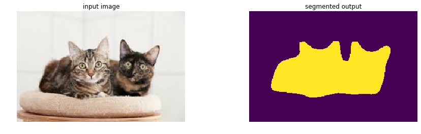

References:

1. Fully Convolutional Networks for Semantic Segmentation
2. U-Net: Convolutional Networks for BiomedicalImage Segmentation
3. Convolution arithmetic
4. Spatial Pyramid Pooling in Deep Convolutional Networks for Visual Recognition
5. DeepLab: Deep Labelling for Semantic Image Segmentation
6. A Basic Introduction to Separable Convolutions