In machine learning, the difference between the predicted output and the actual output is used to tune the parameters of the algorithm. This error in prediction, so called loss, is a crucial part of designing a good model as it evaluates the performance of our model. For accurate predictions, one needs to minimize this loss. In neural networks, it is done using the gradient descent. There are many types loss functions. Some of them are:
L2 loss (Mean-squared error)
Mean squared error is the most common used loss function for regression loss. It minimizes the squared difference between the predicted value and the actual value. The residual sum of squares is defined as:
\[RSS = \sum_{i=1}^n(y_{i} - \hat{y_i})^2\]import numpy as np
def l2_loss(yhat, y):
return np.sum((yhat - y)**2))L1 loss (Mean-absolute error)
L1 loss minimized the sum of absolute error between the predicted value and the actual value.
\[L(y, \hat{y}) = \sum_{i=1}^n \left| y_{i} - \hat{y_i} \right|\]def l1_loss(yhat, y):
return np.sum(np.absolute(yhat - y))Note: L1 and L2 are also used in regularization. Don’t get confused.
Hinge loss
The hinge loss is used for classification problems e.g. in case of suppport vector machines. It is defined as:
\[L(y, \hat{y}) = max(0, 1-\hat{y} * y)\]def hinge(yhat, y):
return np.max(0, 1 - yhat * y)Cross-entropy (log loss)
Background: Entropy
Before understanding cross-entropy, it helps to understand entropy, a concept from information theory introduced by Claude Shannon. Entropy measures the amount of uncertainty or surprise in a probability distribution. For a discrete random variable X with probability distribution p(x), it is defined as:
\[H(X) = -\sum_{x} p(x) \log p(x)\]The term \(-\log p(x)\) represents the “surprise” of observing event x — the less likely an event, the more surprising it is. Entropy is the expected value of this surprise. It is high when probabilities are nearly uniform (high uncertainty) and low when the distribution is skewed (low uncertainty). For example, a fair coin has entropy of 1 bit, while a biased coin that always lands heads has zero entropy.
Cross-entropy extends this concept to measure the difference between two distributions.
Definition
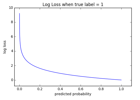
The cross-entropy loss is used in case of classification problems for estimating the accuracy of model whose output is a probability, p, which lies between 0 and 1. In case of binary classification, it can be written as:
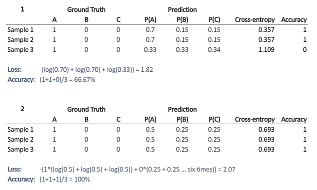
For multi-class classification problems, it is:
\[L(y) = -\sum_{c=1}^n y_{o,c}\log(p_{o,c})\]Here, y is a binary indicator (0 or 1) if class label c is the correct classification for observation o and p is predicted probability observation s.t. o is of class c.
def cross_entropy(y, p):
    return -np.sum(np.multiply(y, np.log(p)) + np.multiply((1-y), np.log(1-p)))
Relationship to KL Divergence
Cross-entropy is closely related to the Kullback-Leibler (KL) divergence, which quantifies the information lost when distribution Q is used to approximate another distribution P:
\[D_{KL}(P \parallel Q) = H(P, Q) - H(P)\]where \(H(P, Q)\) is the cross-entropy and \(H(P)\) is the entropy of the true distribution. Since \(H(P)\) is constant for a fixed dataset, minimizing cross-entropy is equivalent to minimizing the KL divergence between the true and predicted distributions. KL divergence is non-negative and non-symmetric; it equals zero only when \(P = Q\).
Connection to Maximum Likelihood Estimation
Minimizing cross-entropy is equivalent to maximizing the log-likelihood of the data under a Bernoulli (binary) or multinomial (multi-class) model. The negative log-likelihood for a Bernoulli distribution is exactly the binary cross-entropy loss:
\[\theta_{MLE} = \arg\max_{\theta} \log L(\theta \mid x) \equiv \arg\min_{\theta} \text{CE Loss}\]This gives cross-entropy a solid statistical foundation. It is the loss function that yields the Maximum Likelihood Estimate of the model parameters.
For a detailed example using log loss, check logistic regression implementation on GitHub: kHarshit/ML-py.
Conclusion
The choice of loss function depends on the class of problem (regression / classification) as well as is sometimes specific to the problem.
References:
Comments