Our machine learning model often encouters the problem of overfitting. Regularization is one of the techniques to solve this problem.
In regularization, we add the penalty parameter to the cost function so we penalize the model by increasing the penalty for overfitted model.
In linear regression,
we use least squares fitting procedure to estimate regression coefficients \(\beta_{0}, \beta_{1}, \beta_{2}, ..., \beta_{p}\) while minimizing the loss function, residual sum of squares:
Implementing the above model in the dataset fruit_data_with_colors.txt.
PyDev console: using IPython 6.1.0
Python 3.6.3 |Anaconda, Inc.| (default, Nov  3 2017, 19:19:16)
[GCC 7.2.0] on linux
In[2]: import pandas as pd
In[3]: from sklearn.model_selection import train_test_split
In[4]: from sklearn.linear_model import Ridge, Lasso, LinearRegression
In[5]: fruits = pd.read_table('fruit_data_with_colors.txt')
In[6]: fruits.head()
Out[6]:
   fruit_label fruit_name fruit_subtype  mass  width  height  color_score
0            1      apple  granny_smith   192    8.4     7.3         0.55
1            1      apple  granny_smith   180    8.0     6.8         0.59
2            1      apple  granny_smith   176    7.4     7.2         0.60
3            2   mandarin      mandarin    86    6.2     4.7         0.80
4            2   mandarin      mandarin    84    6.0     4.6         0.79
In[7]: X = fruits[['mass', 'width', 'height']]
In[8]: y = fruits[['fruit_label']]
In[9]: X_train, X_test, y_train, y_test = train_test_split(X, y, random_state=0)
In[10]: lm = LinearRegression()
In[11]: lm.fit(X_train, y_train)
Out[11]: LinearRegression(copy_X=True, fit_intercept=True, n_jobs=1, normalize=False)
In[12]: lm.score(X_train, y_train)
Out[12]: 0.72629741095374023
In[13]: lm.score(X_test, y_test)
Out[13]: 0.11996287693912289
This model can overfitt. Some of the regularization techniques are:
Ridge regression
In ridge regression, we use the L2 penalty i.e. adds penalty equivalent to square of the magnitude of coefficients i.e. we minimize
Here, \(\lambda \geq 0\) is known as a tuning parameter. When \(\lambda = 0\), the penalty term has no effect and ridge regression will produce the least square estimates. However, as \(\lambda \rightarrow \infty\), the impact of penalty increases.
NOTE: It is best to apply ridge regression after standarizing the predictors (feature normalization).
In[14]: linreg = Ridge(alpha=20.0)  # alpha is the L2 (regularization) penalty
In[15]: linreg.fit(X_train, y_train)
Out[15]:
Ridge(alpha=20.0, copy_X=True, fit_intercept=True, max_iter=None,
   normalize=False, random_state=None, solver='auto', tol=0.001)
In[16]: linreg.score(X_train, y_train)
Out[16]: 0.52368273228541695
In[17]: linreg.score(X_test, y_test)
Out[17]: 0.31025395205633122
Ridge regression solves the problem of overfitting (high variance) as a consequence of bias-variance tradeoff. As \(\lambda\) increases, the flexibility of regression fit decreases, leading to decreases variance but increased bias.
Lasso regresssion
In lasso regression, we use L1 penalty i.e. adds penalty equivalent to absolute value of the magnitude of coefficients so we minimize
The benefit in lasso regression is that L1 penalty can force some of the coefficient estimates to be exactly equal to \(0\) when \(\lambda\) is large unlike in ridge regression.
Regularization in Neural Networks
In neural networks, there are many regularization techniques used such as L2 regularization (Frobenius norm regularization), Early stopping, Dropout regularization and many more.
In general, there are many regularization techniques. Each has some advantages over others. The choice of regularization technique to use depends on the type of problem you’re trying to solve.
References:
Comments