As discussed in the post linear algebra and deep learning, the optimization is the third and last step in solving image classification problem in deep learning. It helps us find the values of weights W and bias b that minimizes the loss function.
The Strategy
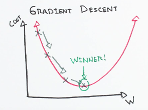
We use the concept of following the gradient to find the optimal pairs of W and b i.e. we can compute the best direction along which we should change our weight vectors that is mathematically guaranteed to be the direction of the steepest descent. This direction is found out by the gradient of the loss function.
Computation
There are two ways to compute the gradient:
- Numerical gradient: The numerical gradient is very simple to compute using the finite difference approximation, but the downside is that it is approximate and that it is very computationally expensive to compute. We use the following expression to calculate numerical gradient:
- Analytical gradient: The second way to compute the gradient is analytically using Calculus, which allows us to derive a direct formula for the gradient (no approximations) that is also very fast to compute.
Unlike the numerical gradient it can be more error prone to implement, which is why in practice it is very common to compute the analytic gradient and compare it to the numerical gradient to check the correctness of your implementation. This is called a gradient check.
Now that we can compute the gradient of the loss function, the procedure of repeatedly evaluating the gradient and then performing a parameter update is called gradient descent.
# basic gradient descent
while True:
    weights_grad = evaluate_gradient(loss_fn, data, weights)  # gradient calculation
    weights += -step_size * weights_grad  # parameter update
This simple loop is at the core of all Neural Network libraries.
Mini-Batch Gradient Descent
When the training data is large, it’s computationally expensive and wasteful to compute the full loss function over the entire training set to perform a single parameter update. Thus, a simple solution of using the batches of training data is implemented. This batch is then used to perform parameter update.
# mini-batch gradient descent
while True:
    data_batch = sample_training_data(data, 256)  # sample training 256 examples
    weights_grad = evaluate_gradient(loss_fn, data_batch, weights)
    weights += -step_size * weights_grad
The extreme case of this is a setting where the mini-batch contains only a single example. This process is called Stochastic Gradient Descent (SGD) (or on-line gradient descent).
Why Gradient Descent Works: Convexity
Gradient descent is guaranteed to find the global minimum when the loss function is convex. A function \(f\) is convex if for any two points \(x_1\) and \(x_2\) and any \(t\) in \([0, 1]\):
\[f(t x_1 + (1-t) x_2) \leq t f(x_1) + (1-t) f(x_2)\]Intuitively, a convex function is bowl-shaped, the line segment between any two points lies above the function. This property ensures any local minimum is also a global minimum. A key consequence is Jensen’s inequality: for a convex function \(\varphi\), the function of the expectation is less than or equal to the expectation of the function:
\[\varphi(\mathbb{E}[X]) \leq \mathbb{E}[\varphi(X)]\]For concave functions (like the log-likelihood), the inequality reverses. Many common loss functions (e.g., MSE, cross-entropy) are convex, which is why gradient descent reliably converges when the learning rate is properly tuned.
Beyond First-Order: The Hessian
Gradient descent is a first-order method, it uses only the gradient (first derivative). The Hessian matrix extends this to second-order information. It is a square matrix of second-order partial derivatives:
\[\mathbf{H}(f) = \begin{bmatrix} \frac{\partial^2 f}{\partial x_1^2} & \frac{\partial^2 f}{\partial x_1 \partial x_2} & \cdots \\ \frac{\partial^2 f}{\partial x_2 \partial x_1} & \frac{\partial^2 f}{\partial x_2^2} & \cdots \\ \vdots & \vdots & \ddots \end{bmatrix}\]The Hessian describes the curvature of the loss function at a point. High curvature means the gradient changes rapidly, so smaller steps are needed. Second-order methods like Newton’s method use the Hessian for more informed updates:
\[w_{t+1} = w_t - \mathbf{H}^{-1} \nabla L(w_t)\]However, computing the Hessian is \(O(n^2)\) per update and its inverse is \(O(n^3)\), making it impractical for large neural networks. This is why first-order methods like gradient descent, requiring only \(O(n)\) per update, remain the workhorse of deep learning.
Conclusion
Gradient descent is one of many optimization methods, namely first order optimizer, meaning, that it is based on analysis of the gradient of the objective. In order to calculate gradients efficiently, we use backpropagation. Consequently, in terms of neural networks it is often applied together with backprop to make an efficient updates.
Read more:
Understanding gradient descent algorithm
References:
image source
Comments