Mathematics lies behind every algorithm; if not mathematics then mathematical thinking. In case of deep learning algorithms, linear algebra is the driving force.
In an image classification problem, we often use neural networks.
The Score Function
The first step in that process is to assign a score function that maps the raw data to class scores i.e. to map the pixel values of an image to the confidence score of each class.
For a given training dataset of images having N examples (each with a dimensionality D) and K distinct categories, we can write mathematically each image as \(x_{i} \in R^D\), each associated with a label \(y_{i}\) where \(i = 1, 2,...n\) and \(y_{i} = 1, 2,...K\). For example, in the famous CIFAR-10 dataset, we have a training set of N = 50,000 images, each with D = 32 x 32 x 3 = 3072 pixels, and K = 10, since there are 10 distinct classes (dog, cat, car, etc).
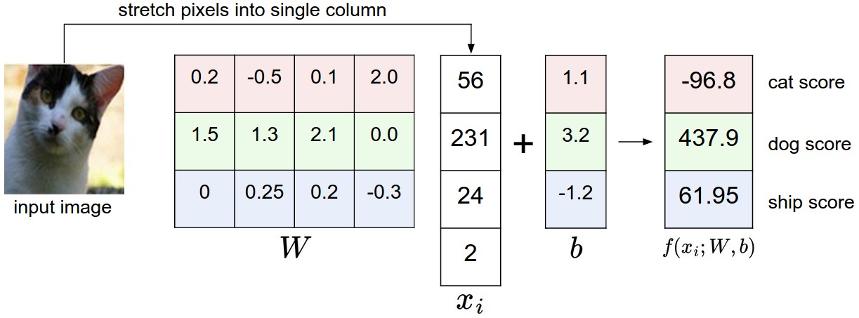
Let’s assume that the image \(x_{i}\) has all of its pixels flattened out in a single column into a vector D x 1. The matrix W (weights) and b (bias vector) are of shape K x D and K x 1 respectively.
We can define the score function which maps the raw images to class scores as \(f : R^D \mapsto R^K\). Let’s take the simple linear function. In Convolutional Neural Networks, we use a complex score function than the one discussed here:
\[f(x_{i}, W, b) = Wx_{i} + b\]For example, in the CIFAR-10 dataset, all pixels in the ith image are flattened into a single 3072 x 1 column vector, W is 10 x 3072 and b is 10 x 1.
In this approach, notice that we don’t have any control over fixed \(x_{i}\) and \(y_{i}\), but we can certainly modify our parameters W and b. Our goal is to set the parameters W and b such that the computed scores match their true values.
Loss and Optimization
Now the question is how do we modify the parameters. We measure the prediction based on the loss fuction which gives a high loss if our model is doing the poor job of classifying the training data. This is the second step in the image classification problem. The loss function can be modified in a way to make good predictions by including a regularization term.
The third and last step to solve image classification problem using neural networks is to optimize the parameters W and b so as to minimize the loss function. For optimization, we use the concept of following the gradient. The algorithm that implements this approach is called gradient descent. We’ll talk about it the next posts.
The linear algebra seen here, matrix multiplication, weight matrices, and transformations, also underpins dimensionality reduction techniques often used in data preprocessing. PCA (Principal Component Analysis) uses eigendecomposition of the covariance matrix or SVD (Singular Value Decomposition) to project high-dimensional data into a lower-dimensional space while preserving variance. SVD factorizes a matrix as \(A = USV^T\) and is more numerically stable than eigendecomposition. These techniques help reduce noise and overfitting before data enters the network.
References:
Convolution Neural Networks for Visual Recognition
Comments