Building neural networks, we compute gradients with the backpropagation algorithm. These gradients are used to perform the parameter updates. The default way of doing this is to update gradient along the negative gradient direction i.e. using the gradient descent optimizer.
# SGD
while True:
    data_batch = sample_training_data(data, 1)  # sample training 1 example
    # gradient calculation
    weights_grad = evaluate_gradient(loss_fn, data_batch, weights)
    # parameter update
weights += -learning_rate * weights_grad 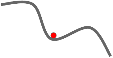
There are certain problems with SGD. If the loss function has a local minima or a saddle point, the gradient becomes zero (gradient descent get stuck).
But, there are many more methods to improve on this. Few of the optimizers are:
Momentum update
Here’s a popular story about momentum: gradient descent is a man walking down a hill. He follows the steepest path downwards; his progress is slow, but steady. Momentum is a heavy ball rolling down the same hill. The added inertia acts both as a smoother and an accelerator, dampening oscillations and causing us to barrel through narrow valleys, small humps and local minima.
— Distill.pub (magazine)
Here, the gradient instead of directly influencing the position, it influences the velocity, which in turn has an effect on the position. The momentum update builds up the velocity in directions having a gentle but consistent gradient.
# momentum update
velocity += mu * velocity - learning_rate * weights_grad  # integrate velocity
weights += velocity  # integrate position
Here, the effect of gradient is to increment the previous velocity. velocity is initialized to zero and value of mu is the rate by which velocity decays, typically taken slightly less than 1. The momentum method has better convergence rate than the basic update.
Nesterov momentum
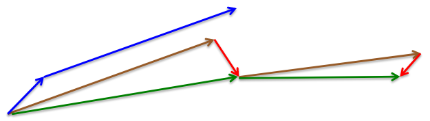
The standard momentum method first computes the gradient at the current position then takes a big jump in the direction of the updated accumulated gradient. While, in Nesterov momentum, first make a big jump in the direction of the previous accumulated gradient then measure the gradient where you end up and make a correction. It has better convergence than the standard momentum.
# momentum update
v_prev = v # back this up
v = mu * v - learning_rate * dx # velocity update stays the same # dx is gradient
x += -mu * v_prev + (1 + mu) * v # position update changes
Learning Rate Decay
Sometimes, the chosen reasonable learning rate can only decrease the error upto a certain value as shown in the figure. In this scenario, it’s useful to decrease the learning rate. It’s accomplished by using learning rate decay e.g. the learning rate can be decreased by half every 7 epochs.
Adagrad
All the above methods manipulate the learning rate globally and equally for all the parameters. Adagrad is an adaptive learning rate method that adaptively (increase or decrease as required) tune the learning rates per parameter.
# adagrad
# Assume the gradient dx and parameter vector x
cache += dx**2
x += - learning_rate * dx / (np.sqrt(cache) + eps)
cache keep track of per-parameter sum of squared gradients. The learning rate will reduce for the weights having high gradients and increase for the weights having small updates.
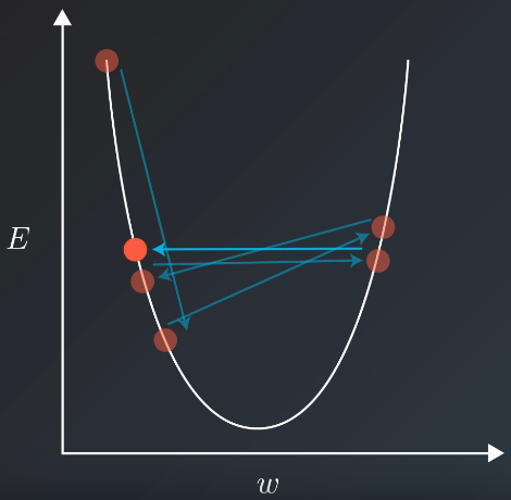
RMSprop
RMSProp keeps a moving average of the root mean squared (rms) gradients, by which we divide the current gradient. This makes the learning process much better.
# rmsprop
cache = decay_rate * cache + (1 - decay_rate) * dx**2
x += - learning_rate * dx / (np.sqrt(cache) + eps)
Adam
Adam is almost similar to RMSProp. Instead of adapting the parameter learning rate based only on the first moment (mean) as in RMSProp, Adam also uses the second moment of the gradients (variance). That is, it calculates the exponential average of the gradient (i.e. mean) and the squared gradient (i.e. variance).
# t is your iteration counter going from 1 to infinity
m = beta1*m + (1-beta1)*dx
mt = m / (1-beta1**t)
v = beta2*v + (1-beta2)*(dx**2)
vt = v / (1-beta2**t)
x += - learning_rate * mt / (np.sqrt(vt) + eps)
The Adam upate also includes the bias correction to compensate the bias at zero of m and v during initialization.
Conclusion
Adam is recommended the default choice of optimization algorithm. However, it’s also worth trying RMSProp and SGD+Nesterov momentum.
References:
- CS231n: Convolutional Neural Networks for Visual Recognition
- Neural Networks for Machine Learning
- Goh, “Why Momentum Really Works”, Distill, 2017. http://doi.org/10.23915/distill.00006
Comments