Contents
In modern deep learning, getting models to train faster and run efficiently in production is a constant challenge. Two key techniques have emerged to address this: Mixed Precision Training (using FP16 alongside FP32 to speed up training) and Quantization (converting FP32 models to INT8 for faster inference). This post walks through the fundamental concepts, practical implementations, and best practices for both.
Part 1: GPUs and Performance
Before diving into mixed precision, it’s essential to understand the hardware and the bottlenecks.
Floating Point Numbers
A floating-point number has three parts:
- Sign bit (1 bit): 0 for positive, 1 for negative.
- Exponent bits: control the range (magnitude).
- Mantissa bits: control the precision.
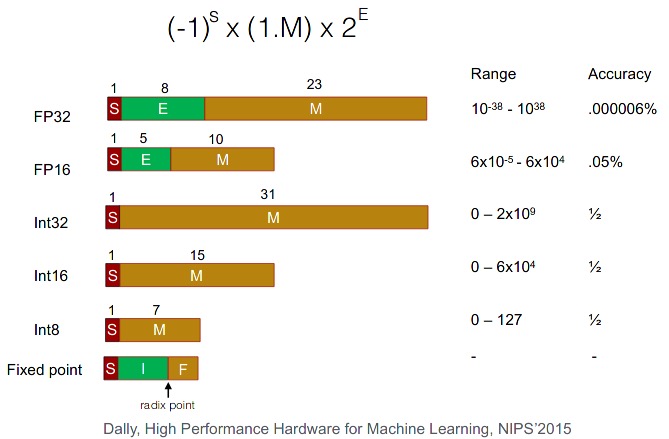
| Type | Total Bits | Exponent Bits | Mantissa Bits | Bias | Use |
|---|---|---|---|---|---|
| FP32 | 32 | 8 | 23 | 127 | Default in C++, PyTorch, TensorFlow |
| FP64 | 64 | 11 | 52 | 1023 | Python float |
| FP16 | 16 | 5 | 10 | 15 | Mixed precision |
The sign bit determines the sign. The 8 exponent bits go from 0 to 255, split into two ranges: 0–126 are negative exponents, 127 represents 0, and 128–255 are positive. The actual exponent value = (exp − 127) for FP32 (bias = 127; for FP64, bias = 1023). The 23 mantissa bits represent decreasing negative powers of 2.
GPU Architecture
- Compute: Streaming Multiprocessors (SMs): the GPU-equivalent of a CPU core (108 SMs on an A100).
- Memory: on-chip L2 cache, and high-bandwidth DRAM (global memory: 40 GB on A100).
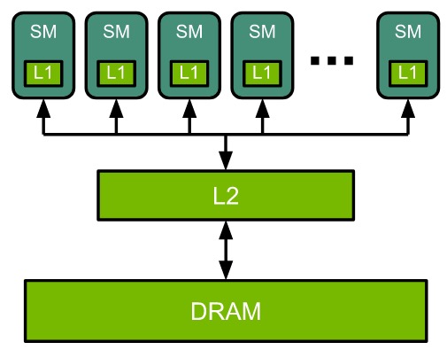
Each SM has a number of CUDA Cores (also called streaming processors, SPs). A single SM can do a certain number of multiply-add (MAC) operations per clock. The MAC operations can be done on either CUDA cores or Tensor Cores. The GPU clock speed indicates how fast the cores run. A 1 GHz processor can do 10⁹ cycles/second. In each cycle, an SM can perform a number of MAC operations.
Peak throughput formula:
\[\text{Peak FP16 throughput} = (\text{# MAC ops/clock/SM} \times \text{# SM} \times \text{SM clock rate}) \times 2\]For NVIDIA A100 (108 SMs, 1.41 GHz clock, 1024 FP16 MAC ops/clock/SM):
\[(1024 \times 2) \times 108 \times (1.41 \times 10^9) \approx 312 \text{ TFLOPS}\]CUDA Programming Model
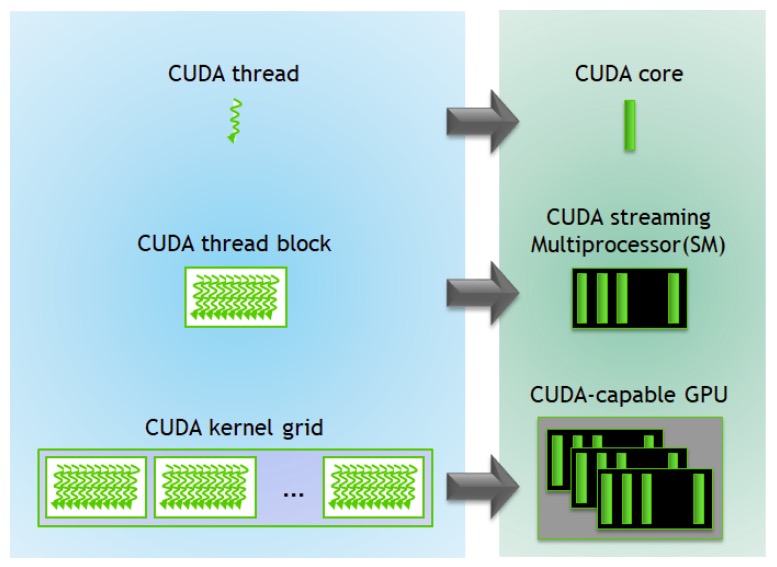
The CUDA programming model provides an abstraction of GPU architecture (API for GPUs).
A CUDA kernel is a function executed by the GPU in parallel. A parallel code (e.g. matmul) is executed n times in parallel by n different CUDA threads.
- Threads are grouped into a CUDA block; CUDA blocks are grouped into a grid.
- Warps (groups of 32 threads) execute simultaneously.
- A kernel is executed as a grid of blocks of threads.
- One SM can run several concurrent CUDA blocks.
- A GPU consists of multiple SMs.
A GPU’s specification (features) is given by its Compute capability (Major.Minor), e.g. NVIDIA A2 has compute capability 8.6.
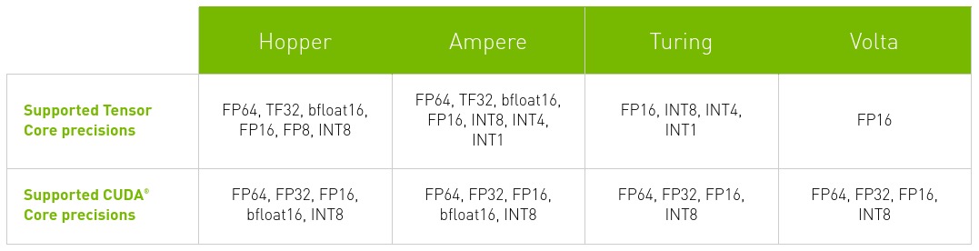
Tensor Cores
Tensor Cores are programmable matrix multiply-and-accumulate (MAC) units that perform fused matrix-multiply-add (FMA) at much higher throughput than CUDA cores, with reduced precisions like FP16, and INT8.
“Tensor Cores are so fast that computation is no longer a bottleneck. The only bottleneck is getting data to the Tensor Cores.”
- CUDA cores perform scalar instructions: multiplication of an element of A with an element of B; perform one MAC operation per GPU clock.
- Tensor Cores perform matrix instructions: multiplication between vectors/matrix of elements at a time; perform a matrix MAC (multiple operations)(
4x4matrix in Volta) per GPU clock.
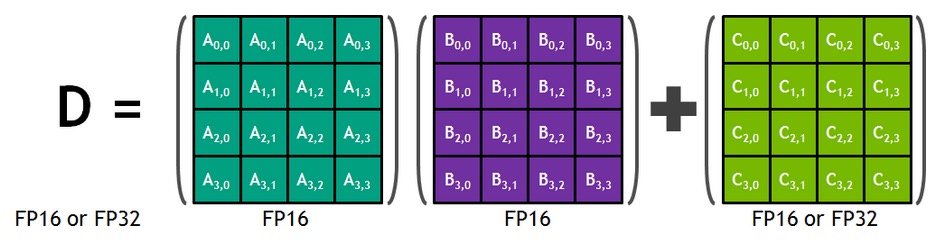
During training with FP16 inputs, Tensor Cores compute products without loss of precision and accumulate in FP32. Note that the operations like element-wise addition of two fp16 tensors, that can’t be formulated in terms of matrix blocks, still use CUDA cores.
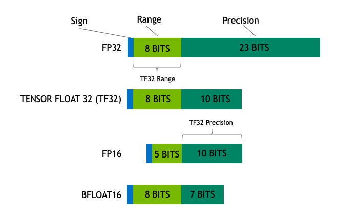
TF32 Mode
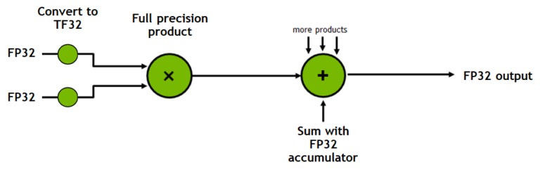
TF32 is a Tensor Core operation mode (not a storage format). It uses the exponent range of FP32 but the mantissa precision of FP16.
- Storage and all other operations remain in FP32.
- Only
convandmatmulconvert inputs to TF32. - It is the default 32-bit format in cuDNN, PyTorch, and TensorFlow on Ampere GPUs.
TF32 vs FP32 in PyTorch
Benchmark on NVIDIA RTX A4000 with 10240×10240 matrix multiplication:
TF32 benchmark (default):
# using tf32 by default for matmul on NVIDIA A4000
avg = 0
n = 10
for i in range(n):
    a = torch.randn(10240, 10240, device='cuda')  # fp32
    b = torch.randn(10240, 10240, device='cuda')  # fp32
    start = timeit.default_timer()
    out = a @ b
    end = timeit.default_timer()
    print(i, ": ", end-start)
    if i>2:
        avg += end-start
print('avg[2:] is ', avg/(n-3))
0 :  0.4807837880216539
1 :  4.059402272105217e-05
2 :  0.00015917990822345018
3 :  1.3931072317063808e-05
4 :  1.3400916941463947e-05
5 :  1.5689991414546967e-05
6 :  1.3425946235656738e-05
7 :  1.3030949048697948e-05
8 :  1.3077049516141415e-05
9 :  1.2170989066362381e-05
avg[2:] is  1.3532416362847601e-05
FP32 benchmark (TF32 disabled):
# disable tf32: use fp32 on NVIDIA A4000
torch.backends.cuda.matmul.allow_tf32 = False
avg = 0
n = 10
for i in range(n):
    a = torch.randn(10240, 10240, device='cuda')  # fp32
    b = torch.randn(10240, 10240, device='cuda')  # fp32
    start = timeit.default_timer()
    out = a @ b
    end = timeit.default_timer()
    print(i, ": ", end-start)
    if i>2:
        avg += end-start
print('avg[2:] is ', avg/(n-3))
0 :  9.770691394805908e-05
1 :  4.72670653834939e-05
2 :  2.1450920030474663e-05
3 :  2.470705658197403e-05
4 :  2.0278035663068295e-05
5 :  1.9971979781985283e-05
6 :  1.930294092744589e-05
7 :  2.001994289457798e-05
8 :  1.9033905118703842e-05
9 :  1.9156024791300297e-05
avg[2:] is  2.035284082272223e-05
Accuracy comparison:
# compare accuracy of tf32 vs fp32 on NVIDIA A4000
a = torch.randn(10240, 10240, device='cuda')  # fp32
b = torch.randn(10240, 10240, device='cuda')  # fp32

torch.backends.cuda.matmul.allow_tf32 = True
mean_tf32 = (a @ b).abs().mean()  # tf32 matmul

torch.backends.cuda.matmul.allow_tf32 = False
mean_fp32 = (a @ b).abs().mean()  # fp32 matmul

print(f'mean: tf32: {mean_tf32}, fp32: {mean_fp32}, diff:{abs(mean_tf32-mean_fp32)}')
mean: tf32: 80.71688079833984, fp32: 80.71910095214844, diff:0.00222015380859375
TF32 delivers ~1.5× speedup (13.5 µs vs 20.4 µs warm) with a mean absolute difference of only 0.0022 — negligible accuracy loss for deep learning workloads.
GPU Sharing & MIG
When individual workloads don’t saturate the GPU (e.g. inference with low batch size, visualization workload), sharing becomes useful. However, different jobs running on the same GPU compete for the same resources; a job consuming larger memory bandwidth starves others.
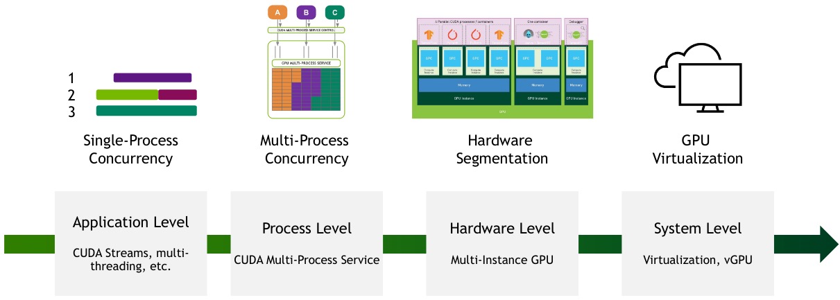
Multi-Instance GPU (MIG) solves this by partitioning a single GPU into separate GPU Instances for CUDA applications, providing multiple users with dedicated GPU resources:
- True hardware isolation
- Guaranteed QoS
- Dedicated resource allocation
- Max GPU utilization
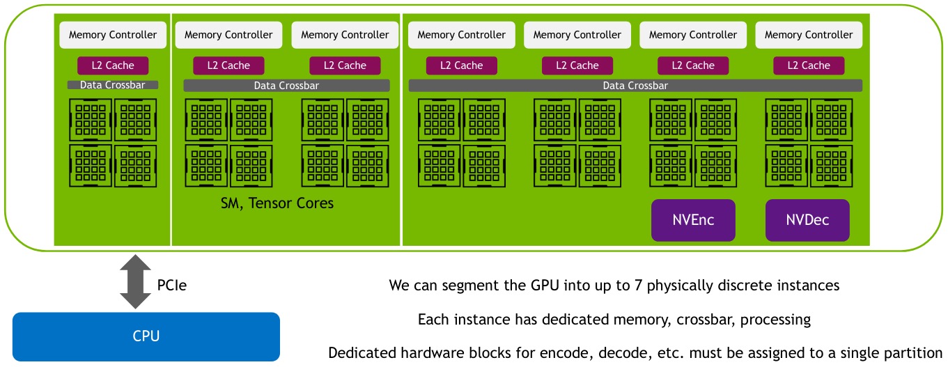
A GPU Instance (GI) is a combination of GPU slices and GPU engines (DMAs, NVDECs, etc.). Everything within a GI shares all GPU memory slices and other GPU engines, but its SM slices can be further subdivided into compute instances (CI).
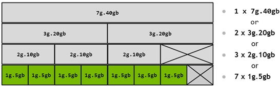
An A100 (40 GB) can be thought of as having 8 × 5 GB memory slices and 7 SM (compute) slices. The number of slices a GI can be created with is not arbitrary, the NVIDIA driver provides GPU Instance Profiles (e.g. MIG 1g.5gb, MIG 2g.10gb).
Performance Analysis
A kernel’s execution time is determined by three factors: math (\(T_{\text{math}}\)), memory (\(T_{\text{mem}}\)), and latency:
\[T_{\text{math}} = \frac{\text{# operations}}{BW_{\text{math}}}, \qquad T_{\text{mem}} = \frac{\text{# bytes accessed}}{BW_{\text{mem}}}\]A kernel is math-limited if \(T_{\text{math}} > T_{\text{mem}}\), i.e.:
\[\frac{\text{# ops}}{\text{# bytes}} > \frac{BW_{\text{math}}}{BW_{\text{mem}}}\]where:
- LHS = arithmetic intensity = # FLOPS / # bytes accessed
- RHS = processor’s ops:byte ratio
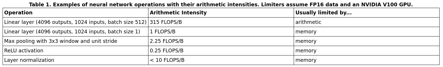
The most likely performance limiter is:
- Latency if there is not sufficient parallelism
- Math-bound: arithmetic intensity > GPU
ops:byteratio (e.g. dot-product operations like matrix-matrix and matrix-vector multiplications in large linear/conv layers with large batch size). - Memory-bound: arithmetic intensity < GPU
ops:byteratio (e.g. element-wise ops like ReLU where few operations per byte are accessed, element-wise addition; reduction ops like pooling, normalization, softmax).
Example: V100 has a peak math rate of 125 FP16 Tensor TFLOPS, an off-chip memory bandwidth of ~900 GB/s, and an on-chip L2 bandwidth of 3.1 TB/s, giving it an ops:byte ratio between 40 and 139, depending on the source of an operation’s data (on-chip or off-chip memory).
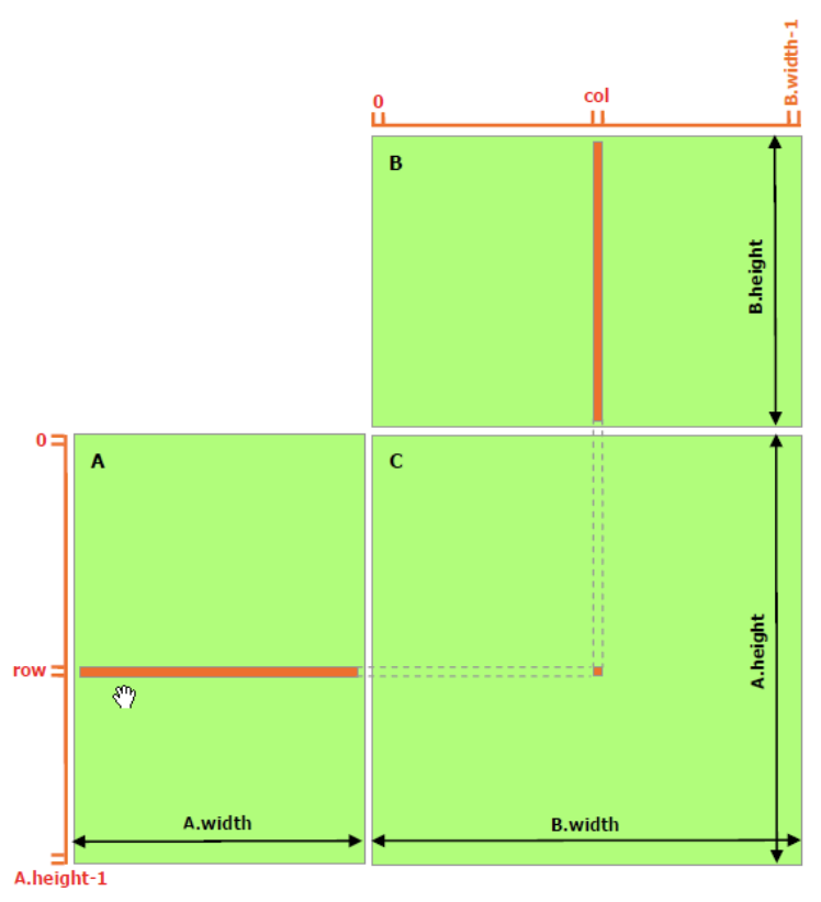
Performance: GEMMs
General Matrix Multiplications (GEMMs) are the building blocks of fully connected, convolutional, and LSTM layers:
\[C = \alpha AB + \beta C\]GEMMs are done in parallel by the GPU by dividing the output matrix into tiles, which are assigned to thread blocks. Each thread block loads values from \(A\) and \(B\), computes the output tile, and accumulates it in the output matrix.
To compute the product, \(M \times N \times K\) fused multiply-adds (FMAs) are needed. Each FMA consists of 2 operations (a multiply and an add):
\[\text{arithmetic intensity} = \frac{2 \times M \times N \times K}{2 \times (M \times K + N \times K + M \times N)}\]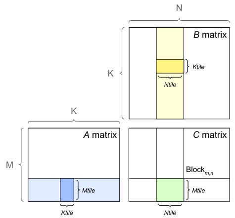
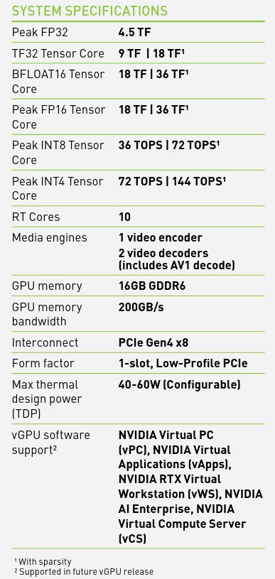
GPU Specifications
- TFLOPS: Tera Floating point Operations Per Second (\(10^{12}\) single-precision floating point operations per second).
- TOPS: Tera Operations (integer, float, etc.) Per Second = # MAC units × frequency of MAC operations × 2.
Part 2: Mixed Precision
What is Mixed Precision?
Mixed precision combines FP32 and FP16 to get the best of both worlds:
- FP32: wide range, higher precision, used where accuracy is critical.
- FP16: smaller range, lower precision, used where speed is critical.
Advantages:
- Speeds up math-intensive operations via FP16 Tensor Cores.
- Speeds up memory-limited operations by halving the bytes accessed.
- Reduces memory requirements, enabling larger models or batch sizes.
Why Not Use FP16 Exclusively?
Problem 1: Underflow in weight updates:
When update / param < 2⁻¹¹ ≈ 0.00049, the update has no effect.
# Imprecise weight update
p = torch.FloatTensor([1.0])
print(p.dtype, p + 0.0001)  # weight += lr*gradient
p = torch.HalfTensor([1.0])
print(p.dtype, p + 0.0001, '-> underflow')
torch.float32 tensor([1.0001])
torch.float16 tensor([1.], dtype=torch.float16) -> underflow
Problem 2 — Overflow in reductions:
a = torch.FloatTensor(4096).fill_(16.0)  # a 4096x1 tensor having each value 16.0
print(a.dtype, a.sum())
a = torch.HalfTensor(4096).fill_(16.0)
print(a.dtype, a.sum(), '-> overflow')
torch.float32 tensor(65536.)
torch.float16 tensor(inf, dtype=torch.float16) -> overflow
Solution: Use FP32 wherever underflow/overflow might happen.
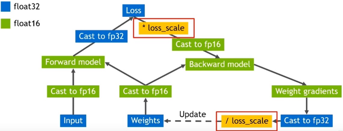
Loss Scaling
In FP16, many activation gradient values become zero because the FP16 range is sufficient but much of it is left unused.
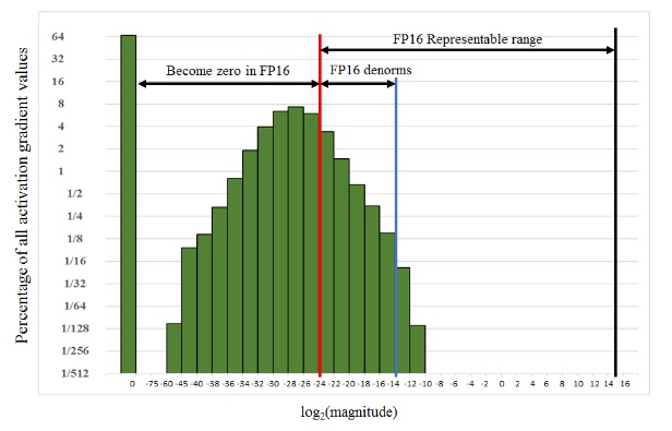
Solution: Scale the gradients to the right to keep them from becoming 0s in FP16 e.g. shift by 15 (multiply by 32k) exponent values in above case. During training, we can multiply the loss by a scaling factor S before backpropagation, then unscale the gradients before the weight update.
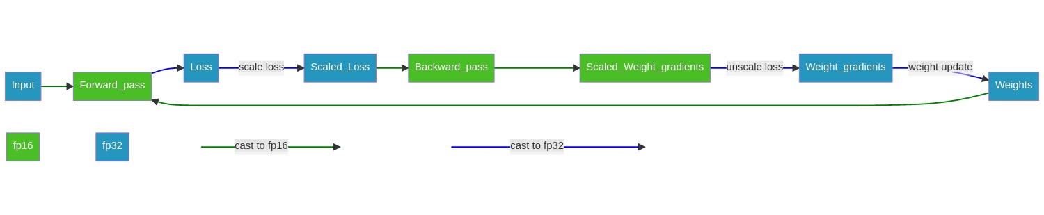
Mixed Precision Training Procedure
- Maintain a primary copy of weights in FP32.
- Initialize loss scaling factor S to a large value.
- For each iteration:
- Make an FP16 copy of weights.
- Forward propagation (FP16 weights and activations).
- Multiply loss by scaling factor S.
- Backward propagation (FP16 weights, activations, and their gradients).
- If Inf/NaN in gradients (overflow due to large S) → reduce S, skip update and move to next iteration.
- Unscale gradients (× 1/S).
- Weight update in FP32 (including gradient clipping, weight decay etc.).
- If no Inf/NaN for N iterations → increase S.
Automatic Mixed Precision (AMP)
AMP automates three tasks:
- Automatic casting between FP16 and FP32.
- Automatic loss scaling to preserve small gradient values.
- FP32 Master weight management in the optimizer to accumulate per-iteration weight updates.
Operation casting rules:
| Operation Type | Examples | Limiter | Precision |
|---|---|---|---|
| Dot-product ops | matmul, conv, linear | Math-bound | computation in FP16, accumulate partial product in FP32 |
| Element-wise ops | ReLU, addition | Memory-bound | FP32 |
| Reduction ops | pooling, softmax, norm | Memory-bound | FP32 |
| Autocasting Behaviour | Ops |
|---|---|
| Ops autocast to fp16 | matmul, linear, conv2d, LSTMCell, etc. |
| Ops autocast to fp32 | pow, sum, normalize, softmax, etc. |
AMP in PyTorch
AMP can be used in PyTorch as follows.
def train(n_epochs, loaders, model, optimizer, criterion, use_amp=False):
    scaler = torch.cuda.amp.GradScaler(enabled=use_amp)  #1 initialize gradient scaler
    for epoch in range(1, n_epochs+1):
        train_loss, valid_loss = 0.0, 0.0
        model.train()  # set model to training mode
        torch.cuda.synchronize()
        start_time = time.time()

        for batch_idx, (data, target) in enumerate(loaders['train']):
            data, target = data.to(device), target.to(device)
            optimizer.zero_grad()
            with torch.cuda.amp.autocast(enabled=use_amp):  #2 use AMP context
                outputs = model(data)  # forward pass
                loss = criterion(outputs, target)
            scaler.scale(loss).backward()  #3 call backward pass on scaled loss
            scaler.step(optimizer)  #4 unscale gradients, do weight update if not Infs or NaNs
            scaler.update()  #5 update scale factor for next iteration
            train_loss += ((1 / (batch_idx + 1)) * (loss.item() - train_loss))

        model.eval()
        for batch_idx, (data, target) in enumerate(loaders['valid']):
            data, target = data.to(device), target.to(device)
            with torch.no_grad():
                with torch.cuda.amp.autocast(enabled=use_amp):  # AMP
                    outputs = model(data)
                    loss = criterion(outputs, target)
                valid_loss += ((1 / (batch_idx + 1)) * (loss.item() - valid_loss))
        torch.cuda.synchronize()
        end_time = time.time()
        total_time = round((end_time - start_time)/60, 2)
        print(f'Epoch: {epoch} \tTraining Loss: {train_loss:.3f} \tValidation Loss: {valid_loss:.3f} \tTime: {total_time}min')

    return model
FP32 training (NVIDIA GeForce RTX 2060 SUPER, Turing, trainable layers: fc of resnet101, 4 params):
print('FP32 training')
start_timer()
model_fp32 = train(5, loaders, model, optimizer, criterion, use_amp=False)
fp32_time, fp32_mem = end_timer_and_print()
fp32_accuracy = test(loaders['test'], model_fp32)
FP32 training
Epoch: 1 	Training Loss: 3.759 	Validation Loss: 1.997 	Time: 0.55min
Epoch: 2 	Training Loss: 1.859 	Validation Loss: 0.936 	Time: 0.58min
Epoch: 3 	Training Loss: 1.309 	Validation Loss: 0.676 	Time: 0.55min
Epoch: 4 	Training Loss: 1.127 	Validation Loss: 0.595 	Time: 0.55min
Epoch: 5 	Training Loss: 1.079 	Validation Loss: 0.501 	Time: 0.57min
Total execution time: 2.81 min
Max memory: 2876.02 MiB
Test Accuracy: 84% (710/836)
AMP training (same setup):
print('AMP training')
start_timer()
model_amp = train(5, loaders, model, optimizer, criterion, use_amp=True)
amp_time, amp_mem = end_timer_and_print()
amp_accuracy = test(loaders['test'], model_amp)
AMP training
Epoch: 1 	Training Loss: 3.771 	Validation Loss: 1.993 	Time: 0.5min
Epoch: 2 	Training Loss: 1.858 	Validation Loss: 0.910 	Time: 0.48min
Epoch: 3 	Training Loss: 1.312 	Validation Loss: 0.673 	Time: 0.5min
Epoch: 4 	Training Loss: 1.124 	Validation Loss: 0.558 	Time: 0.48min
Epoch: 5 	Training Loss: 1.049 	Validation Loss: 0.484 	Time: 0.5min
Total execution time: 2.45 min
Max memory: 1798.03 MiB
Test Accuracy: 84% (709/836)
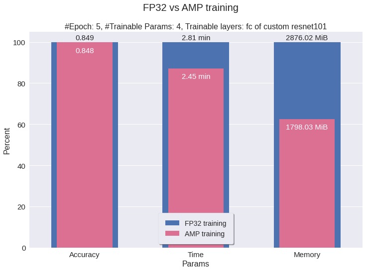
| Metric | FP32 | AMP | Improvement |
|---|---|---|---|
| Total Time | 2.81 min | 2.45 min | 13% faster |
| Peak Memory | 2876 MB | 1798 MB | 37% less |
| Test Accuracy | 84% | 84% | Same accuracy |
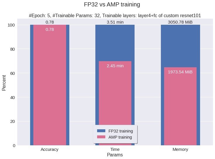
In above example, we only trained 4 params, if we increase the number of params, we’d see more improvement in time and memory saving.
AMP in TensorFlow
# 1. set mixed precision policy
policy = mixed_precision.Policy('mixed_float16')
mixed_precision.set_global_policy(policy)

# Computations are done in float16 for performance, but variables must be kept in float32 for numeric stability
print(f'Compute dtype: {policy.compute_dtype}')
print(f'Variable dtype: {policy.variable_dtype}')
# 2. initialize loss scaler
loss_object = tf.keras.losses.SparseCategoricalCrossentropy()
optimizer = keras.optimizers.RMSprop()
optimizer = mixed_precision.LossScaleOptimizer(optimizer)

@tf.function
def train_step(x, y):
    with tf.GradientTape() as tape:
        predictions = model(x)  # forward pass
        loss = loss_object(y, predictions)
        scaled_loss = optimizer.get_scaled_loss(loss)  # 3. scale loss
    scaled_gradients = tape.gradient(scaled_loss, model.trainable_variables)  # 4. get scaled gradients
    gradients = optimizer.get_unscaled_gradients(scaled_gradients)  # 5. unscale gradients
    optimizer.apply_gradients(zip(gradients, model.trainable_variables))  # 6. weight update
    # also updates the loss scale, halving it if gradients had Infs or NaNs
    return loss

@tf.function
def test_step(x):
    return model(x, training=False)
Conclusion on Mixed Precision
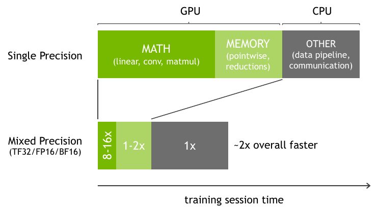
Use AMP. It delivers:
- 1.5–3× speedup on Tensor Core GPUs
- Up to 2× memory savings
- No loss in accuracy for most models
Part 3: Quantization
Quantization converts continuous floating-point numbers to discrete integer representations, enabling faster inference on integer-only hardware.
What is Quantization?
Formal definition:
\[\begin{aligned} r_q &= \text{round}\!\left(\frac{\text{clip}(r, [\alpha, \beta])}{s} + z\right) \\[6pt] s &= \frac{\beta - \alpha}{\beta_q - \alpha_q} \quad (\text{scale}) \\[6pt] z &= \text{zero-point (shift)} \\[6pt] r_{dq} &= (r_q - z) \times s \quad (\text{dequantization}) \\[6pt] \text{Quantization error} &= r - r_{dq} \end{aligned}\]where \(r \in \mathbb{R}\) is the floating-point input, \(r_q\) is the quantized integer value, \(s\) (scale) and \(z\) (zero point) are q-params.
\([\alpha, \beta]\) is the input clipping range, \([\alpha_q, \beta_q]\) is the output integer range, and \(r_{dq}\) is the dequantized value.
Example (unsigned [0, 255]):
\[\begin{bmatrix} 0.34 & 3.75 \\ -4.7 & 0.68 \end{bmatrix}_{\text{FP32 (pre-quant)}} \xrightarrow[]{\text{unsigned [0,255] quantize}} \begin{bmatrix} 64 & 134 \\ 3 & 81 \end{bmatrix}_{\text{INT8 (quant)}} \xrightarrow[]{\text{dequantize}} \begin{bmatrix} 0.41 & 3.62 \\ -4.5 & 0.71 \end{bmatrix}_{\text{FP32 (dequant)}}\]Example (signed [-128, 127]):
\[\begin{bmatrix} -1.54 & 0.22 \\ -0.26 & 2.0 \end{bmatrix}_{\text{FP32 (pre-quant)}} \xrightarrow[]{\text{signed [-128,127] quantize}} \begin{bmatrix} -5 & 1 \\ -1 & 7 \end{bmatrix}_{\text{INT8 (quant)}} \xrightarrow[]{\text{dequantize}} \begin{bmatrix} -1.43 & 0.28 \\ -0.28 & 2.0 \end{bmatrix}_{\text{FP32 (dequant)}}\]Symmetric (Scale) Quantization
- Quantize 0-symmetric dynamic range of floating-point values, i.e.
z = 0(real 0.0 maps to quantized 0), e.g. [-4.2, 4.2] → [-10, 10]. - Clipping range is symmetric:
[−c, c]. - Used primarily for weights.
where \(s\) is the scale factor, \(c\) is the clipping threshold, and \(c = \beta = -\alpha\). The scale is computed as:
\[s = \frac{\beta - \alpha}{\beta_q - \alpha_q} = \frac{2.0 - (-2.0)}{7 - (-7)} = 0.285\]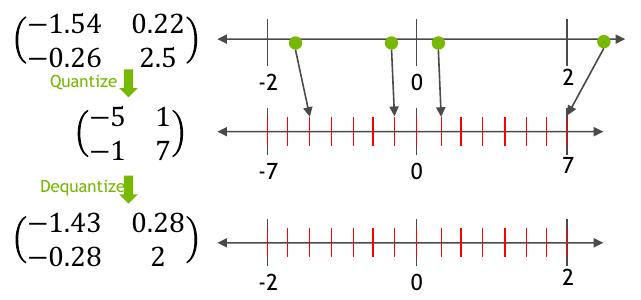
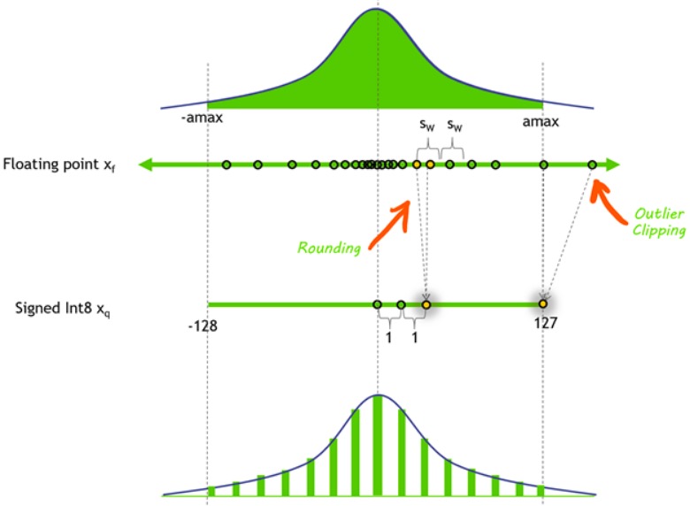
Symmetric Quantization: Full-range vs Restricted-range
\[\text{scale, } s = \frac{\text{input fp32 clip range}}{\text{output int8 range}} = \frac{\beta - \alpha}{\beta_q - \alpha_q}\]- Full-range int8 symmetric quantization: range [-128, 127], \(s = \frac{\beta - \alpha}{2^8 - 1}\)
- Restricted-range int8 symmetric quantization: range [-127, 127], \(s = \frac{\beta - \alpha}{2^8 - 1 - 1}\)
Quantization bias in full-range quantization:
\[A = [-2.2, -1.1, 1.1, 2.2], \; B = [0.5, 0.3, 0.3, 0.5]^T, \; AB = 0\]Full quantization: \(A_q = [-128, -64, 64, 127], \; B_q = [127, 77, 77, 127]^T, \; AB_q = -127 \rightarrow AB_{dq} = -0.00853\), bias introduced
Restricted quantization: \(A_q = [-127, -64, 64, 127], \; B_q = [127, 76, 76, 127]^T, \; AB_q = 0 \rightarrow AB_{dq} = 0\), no bias
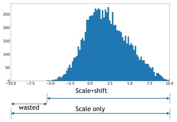
Asymmetric (Affine / Scale+Shift) Quantization
- Quantize arbitrary range of fp32 values, e.g. [-4.0, 8.3] → [0, 10].
- Zero-point
z ≠ 0(real 0.0 maps to quantizedz). The shift byzensuresfloat(0.0) == int(0)because 0 occurs frequently otherwise errors may accumulate. - Clipping range is arbitrary:
[α, β]. - Used primarily for activations.
- Slightly more accurate but requires more compute.
where \(s\) is the scale factor, \(z\) is the zero-point (shift), and \([\alpha, \beta]\) are the clipping thresholds.

Range Calibration: Static vs Dynamic
Calibration is the process of choosing the clipping range \([\alpha, \beta]\) of input fp32 values thus computing q-params.
Static Quantization: clipping range is pre-calculated once before inference (faster).
Dynamic Quantization: range is computed at runtime (more accurate but slower).
| Entity | Preferred Method |
|---|---|
| Weights | Static (fixed) |
| Activations | Static (faster) or Dynamic (more accurate) |
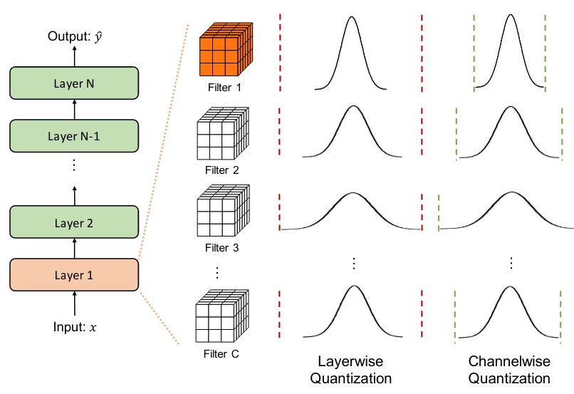
Layer-wise vs Channel-wise Quantization
- Layer-wise (Per-Tensor): one scale/zero-point for the entire weight tensor, used for activations.
- Channel-wise (Per-Channel/Per-Axis): separate q-params per output channel, used for convolutional filters.
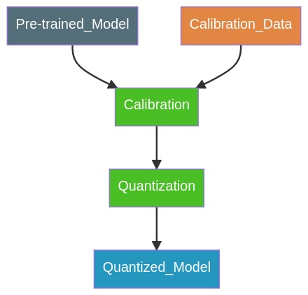
Post-Training Quantization (PTQ): Static
- Weights are quantized prior to inference.
- Activations are quantized using q-params computed from a calibration dataset (unlabeled).
- No fine-tuning required.
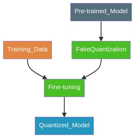
Quantization-Aware Training (QAT): Static
In QAT, the q-params are learned during fine-tuning.
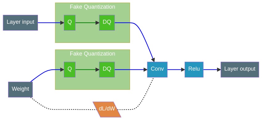
- FakeQuantization nodes (Q/DQ) are inserted during training, (fake as it quantize and immediately dequantize the data adding quantization errors).
- Forward pass:
r_out = DeQuant(Quant(r)). - Backward pass: as usual, gradients pass through unchanged.
- Training loss accounts for quantization effects, producing FP32 weights such that INT8 conversion can maintain accuracy.
Layer Fusion
Fused layers execute in a single kernel call, reducing launch overhead, compared to separate kernel calls for separate layers.
-
Conv + BatchNorm
\[\begin{align} Y &= W * X + b \tag{Conv} \\ Z &= \gamma \frac{Y - \mu}{\sqrt{\sigma^2 + \epsilon}} + \beta \tag{BatchNorm} \\ &= \Big( \frac{\gamma}{\sqrt{\sigma^2 + \epsilon}} W \Big) * X + \bigg( \beta + \frac{\gamma}{\sqrt{\sigma^2 + \epsilon}} (b - \mu) \bigg) \\ &= W' * X + b' \tag{Fused} \end{align}\] - Conv + ReLU
- ReLU + ReLU
- Conv + Pooling, etc.
Quantization Summary
| Quantization Mode | Q-params Calculation | Data Requirements | Speed | Accuracy Loss | Use Case |
|---|---|---|---|---|---|
| PTQ (Dynamic) | Weights: pre-calculated Activations: runtime |
None | ++ | – – | Dynamic models (LSTM) |
| PTQ (Static) | Both pre-calculated | Unlabeled calibration | +++ | – – | All |
| QAT (Static) | Both pre-calculated | Labeled fine-tuning | +++ | – | All |
Conclusion
| Technique | When to Use | Key Benefit |
|---|---|---|
| Automatic Mixed Precision (AMP) | Training | Up to 2× faster, up to 2× memory savings, no accuracy loss |
| Post-Training Quantization (PTQ) | Inference without fine-tuning | 2–4× smaller, 2–4× faster |
| Quantization-Aware Training (QAT) | Inference with highest accuracy | Near-lossless INT8 inference |
References:
- Nvidia Blog and docs