It’s unbelievable how much you don’t know about the game you’ve been playing all your life. — Mickey Mantle
Moneyball tells the story of Oakland A’s in 20021. It was one of the poorest teams in baseball. Billy Beane became its General Manager in 1997. The team’s performance started to improve. But, in the beginning of 2002, Oakland A’s lost three key players. Could they continue improving?
Billy Beane, with his colleague Paul DePodesta, followed an analytical, sabermetric approach to assembling a competitive baseball team, despite Oakland’s disadvantaged revenue situation. Their analysis suggested that some skills were undervalued and some skills were overvalued. If they could detect the undervalued skills, they could find players at a bargain.
The Problem
They analyzed that a team needs to win atleast 95 games to make to the playoffs. Based on this, the A’s calculated that they must score 135 more runs than they allow during the regular season to expect to win 95 games. We can verify this using linear regression. I’m going to use R. The dataset2 baseball.csv consists of 15 variables, whose description is given in codebook.
# read in data
> baseball = read.csv("baseball.csv")
> str(baseball)
'data.frame':	1232 obs. of  15 variables:
 $ Team        : Factor w/ 39 levels "ANA","ARI","ATL",..: 2 3 4 5 7 8 9 10 11 12 ...
 $ League      : Factor w/ 2 levels "AL","NL": 2 2 1 1 2 1 2 1 2 1 ...
 $ Year        : int  2012 2012 2012 2012 2012 2012 2012 2012 2012 2012 ...
 $ RS          : int  734 700 712 734 613 748 669 667 758 726 ...
 $ RA          : int  688 600 705 806 759 676 588 845 890 670 ...
 $ W           : int  81 94 93 69 61 85 97 68 64 88 ...
 $ OBP         : num  0.328 0.32 0.311 0.315 0.302 0.318 0.315 0.324 0.33 0.335 ...
 $ SLG         : num  0.418 0.389 0.417 0.415 0.378 0.422 0.411 0.381 0.436 0.422 ...
 $ BA          : num  0.259 0.247 0.247 0.26 0.24 0.255 0.251 0.251 0.274 0.268 ...
 $ Playoffs    : int  0 1 1 0 0 0 1 0 0 1 ...
 $ RankSeason  : int  NA 4 5 NA NA NA 2 NA NA 6 ...
 $ RankPlayoffs: int  NA 5 4 NA NA NA 4 NA NA 2 ...
 $ G           : int  162 162 162 162 162 162 162 162 162 162 ...
 $ OOBP        : num  0.317 0.306 0.315 0.331 0.335 0.319 0.305 0.336 0.357 0.314 ...
 $ OSLG        : num  0.415 0.378 0.403 0.428 0.424 0.405 0.39 0.43 0.47 0.402 ...
# we're interested only in years before moneyball (2002)
> moneyball = subset(baseball, Year < 2002)
> table(moneyball$W, moneyball$Playoffs)

       0  1
  40   1  0
  50   1  0
  51   1  0
  52   2  0
  53   3  0
  54   5  0
  55   1  0
  56   3  0
  57   5  0
  59   7  0
  60   7  0
  61   6  0
  62   8  0
  63  10  0
  64  13  0
  65  17  0
  66  11  0
  67  19  0
  68  15  0
  69  18  0
  70  17  0
  71  20  0
  72  20  0
  73  22  0
  74  27  0
  75  27  0
  76  36  0
  77  31  0
  78  17  0
  79  32  0
  80  26  0
  81  28  0
  82  20  1
  83  35  0
  84  28  2
  85  30  1
  86  31  1
  87  27  1
  88  23  7
  89  22  5
  90  17 12
  91  15 10
  92  12 11
  93   6  7
  94   6  6
  95   5 15
  96   3  8
  97   4 13
  98   4 11
  99   1  7
  100  1  5
  101  0  7
  102  1  8
  103  1  5
  104  0  4
  106  0  1
  108  0  3
  109  0  1
  114  0  1
  116  0  1
Thus, A team having atleast 95 wins has almost always got into the playoffs, which is in accordance of what DePosta predicted.
# Compute Run Difference (RD) add it to dataframe
> moneyball$RD = moneyball$RS - moneyball$RA
> names(moneyball)  # Note that moneyball now has a new variable 'RD'
 [1] "Team"         "League"       "Year"         "RS"           "RA"
 [6] "W"            "OBP"          "SLG"          "BA"           "Playoffs"
[11] "RankSeason"   "RankPlayoffs" "G"            "OOBP"         "OSLG"
[16] "RD"
# Scatterplot to check for linear relationship
> plot(moneyball$RD, moneyball$W, xlab = "Run Difference", ylab = "Wins", title("Moneyball: Relationship b/w Wins and RD"))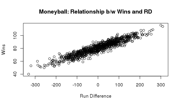
The above plot shows linear relationship b/w Wins and Run Difference.
Now, let’s build our regression model.
# Regression model to predict wins:
> Wins = lm(W ~ RD, data=moneyball)
> summary(Wins)

Call:
lm(formula = W ~ RD, data = moneyball)

Residuals:
     Min       1Q   Median       3Q      Max
-14.2662  -2.6509   0.1234   2.9364  11.6570

Coefficients:
             Estimate Std. Error t value Pr(>|t|)
(Intercept) 80.881375   0.131157  616.67   <2e-16 ***
RD           0.105766   0.001297   81.55   <2e-16 ***
---
Signif. codes:  0 ‘***’ 0.001 ‘**’ 0.01 ‘*’ 0.05 ‘.’ 0.1 ‘ ’ 1

Residual standard error: 3.939 on 900 degrees of freedom
Multiple R-squared:  0.8808,	Adjusted R-squared:  0.8807
F-statistic:  6651 on 1 and 900 DF,  p-value: < 2.2e-16
The regression output includes several important statistics.
The t-statistic for each coefficient is calculated as the ratio of the estimated coefficient to its standard error (e.g., for RD: 0.105766 / 0.001297 = 81.55). It tests the null hypothesis that the specific coefficient is zero, that the predictor has no real effect. A large absolute t-value produces a very small p-value (< 2e-16), which means we reject the null and conclude that Run Difference is significantly associated with Wins.
The F-statistic (6651 on 1 and 900 degrees of freedom) tests the broader null hypothesis that all model coefficients (except the intercept) are simultaneously zero:
\[F = \frac{\text{variation explained by the model}}{\text{variation not explained by the model}}\]A large F-statistic with a tiny p-value (< 2.2e-16) confirms the model as a whole is statistically significant.
Our regression equation for wins is:
W = 80.8814 + 0.105766 × RD and W >= 95
⇒ 95 >= 80.8814 + 0.105766 × RD
⇒ RD = 133.4
Thus, a team need to score almost 135 more pts than allowed to get into the playoffs.
Predicting Runs Scored
Now, how does the A’s score more runs?
The A’s discovered that two baseball statistics were significantly more important than others:
- On-Base percentage (OBP): Percentage of time a player gets on base (including walks) and
- Slugging percentage (SLG): How far a player gets around the bases on his turn (measures power).
And, Batting Average was overvalued. Let’s verify this:
# Regression model to predict runs scored:
> RunsScored = lm(RS ~ OBP + SLG, data=moneyball)
> summary(RunsScored)

Call:
lm(formula = RS ~ OBP + SLG, data = moneyball)

Residuals:
    Min      1Q  Median      3Q     Max
-70.838 -17.174  -1.108  16.770  90.036

Coefficients:
            Estimate Std. Error t value Pr(>|t|)
(Intercept)  -804.63      18.92  -42.53   <2e-16 ***
OBP          2737.77      90.68   30.19   <2e-16 ***
SLG          1584.91      42.16   37.60   <2e-16 ***
---
Signif. codes:  0 ‘***’ 0.001 ‘**’ 0.01 ‘*’ 0.05 ‘.’ 0.1 ‘ ’ 1

Residual standard error: 24.79 on 899 degrees of freedom
Multiple R-squared:  0.9296,	Adjusted R-squared:  0.9294
F-statistic:  5934 on 2 and 899 DF,  p-value: < 2.2e-16
In this multiple regression model, the F-statistic of 5934 (p < 2.2e-16) tests whether at least one of the predictors (OBP or SLG) has a non-zero coefficient. The individual t-statistics for OBP (30.19) and SLG (37.60) are both very large with tiny p-values, confirming both On-Base Percentage and Slugging Percentage are significant predictors of runs scored. The linear regression yields a R-squared value of 0.92, thus our model is a good fit; and both variables are significant.
Runs Scored (RS) = -804.63 + 2737.77(OBP) + 1584.91(SLG) …(i)
Predicting Runs Allowed
We can use pitching statistics to predict runs allowed:
- Opponents On-Base percentage (OOBP)
- Opponents Slugging percentage (OSLG)
We get the linear regression model as:
# Regression model to predict runs allowed:
> RunsAllowed = lm(RA ~ OOBP + OSLG, data=moneyball)
> summary(RunsAllowed)

Call:
lm(formula = RA ~ OOBP + OSLG, data = moneyball)

Residuals:
    Min      1Q  Median      3Q     Max
-82.397 -15.178  -0.129  17.679  60.955

Coefficients:
            Estimate Std. Error t value Pr(>|t|)
(Intercept)  -837.38      60.26 -13.897  < 2e-16 ***
OOBP         2913.60     291.97   9.979 4.46e-16 ***
OSLG         1514.29     175.43   8.632 2.55e-13 ***
---
Signif. codes:  0 ‘***’ 0.001 ‘**’ 0.01 ‘*’ 0.05 ‘.’ 0.1 ‘ ’ 1

Residual standard error: 25.67 on 87 degrees of freedom
  (812 observations deleted due to missingness)
Multiple R-squared:  0.9073,	Adjusted R-squared:  0.9052
F-statistic: 425.8 on 2 and 87 DF,  p-value: < 2.2e-16
Runs Allowed (RA) = -837.38 + 2913.60(OOBP) + 1514.29(OSLG) …(ii)
Results
We can predict how many games the 2002 A’s will win using our models. Using 2001 regular season statistics,
- Team OBP is 0.339 and
- Team SLG is 0.430.
Thus putting these values in the equation (i), we get Runs Scored (RS) = 805.
In the same way, Runs Allowed (RA) = 622 using equation (ii) as in 2001,
- Team OOBP was 0.307 and
- Team OSLG was 0.373.
Now, our regression equation to predict wins was: W = 80.8814 + 0.1058 × RD where RD = RS - RA.
Our prediction for wins in 2002 is: W = 80.8814 + 0.1058(805 – 622) = 100
Paul DePosta used a similar approach to make predictions.
| Our prediction | Paul’s prediction | Actual | |
|---|---|---|---|
| Runs Scored | 805 | 800-820 | 653 |
| Runs Allowed | 622 | 650-670 | 653 |
| Wins | 100 | 93-97 | 103 |
Our prediction closely match actual performace. The A’s set a League record by winning 20 games in a row and made it to the playoffs. Their 2002 record of 103-59 was joint best in Major League Baseball.
Although they didn’t win the World Series, Paul and Billy revolutinised the game through their data-driven approach. Neverthless, Moneyball changed the way many major league front offices do business.
Footnotes:
1: Moneyball ↩
2: Baseball-Reference ↩
3: R (programming language)
Resources:
The case study is an extract of chapter 2 Linear Regression from the Course The Analytics Edge.
Comments