Read the first part The Bayesian Thinking - I and the second part The Bayesian Thinking - II.
There’s no theorem like Bayes’ theorem
Like no theorem we know
Everything about it is appealing
Everything about it is a wow
Let out all that a priori feeling
You’ve been concealing right up to now!
— George Box
In this post, we’ll do probabilistic programming in PyMC31, a python library for programming Bayesian analysis. We’ll discuss the Bayesian view of linear regression.
Frequentist Linear Regression
In Frequentist Linear Regression,
\[\hat{Y} = \hat{β_{0}} + \hatβ_{1}X_{1} + \hatβ_{2}X_{2} + ... + \hatβ_{p}X_{p}\] \[Y = \hat{Y} + \epsilon = β^T X + \epsilon\]we use least squares fitting procedure to estimate regression coefficients \(\beta_{0}, \beta_{1}, \beta_{2}, ..., \beta_{p}\) while minimizing the loss function using residual sum of squares:
\[RSS = \sum_{i=1}^n(y_{i} - \hat{y_i})^2 = \sum_{i=1}^n(y_{i} - β^T x_{i})^2\]We calculate the maximum liklihood estimate of β, the value that is the most probable for X and y.
\[\hat{β} = (X^T X)^{-1} X^T y\]This method of fitting the model parameters is called Ordinary Least Squares (OLS). We obtain a single estimate for the model parameters based on the training data.
Bayesian Linear Regression
In the Bayesian view, the response, y, is not estimated as a single value, but is drawn from a probability distribution.
where \(\sigma\) represents the observation error.
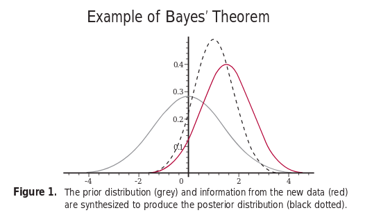
The response, y is generated from a normal (Gaussian) distribution. In Bayesian linear regression, we determine the posterior distribution of model parameters rather than finding a single best value as in frequentist approach. Using the Bayes theorem, the posterior probability of parameters is given by
We include the guess, of what the parameters’ value can be, in our model, unlike the frequentist approach where everything comes from the data. If we don’t have any estimates, we can non-informative priors such as normal distribution.
import pymc3 as pm
import numpy as np
import matplotlib.pyplot as plt

# true parameter values
alpha, sigma = 1, 1
beta = [1, 2.5]

# size of dataset
size = 100

# predictor variable
X1 = np.random.randn(size)
X2 = np.random.randn(size) * 0.2

# simulate response variable
Y = alpha + beta[0]*X1 + beta[1]*X2 + np.random.randn(size)*sigma

fig, axes = plt.subplots(1, 2, sharex=True, figsize=(10, 4))
axes[0].scatter(X1, Y)
axes[1].scatter(X2, Y)
axes[0].set_ylabel('Y')
axes[0].set_xlabel('X1')
axes[1].set_xlabel('X2')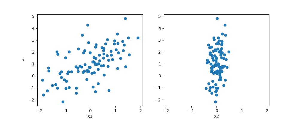
# creates new Model object
basic_model = pm.Model()

with basic_model:
    # objects introduced here are added to the model behind the scenes

    # create stochastic random variables with Normal prior distributions
    alpha = pm.Normal('alpha', mu=0, sd=10)  # intercept
    beta = pm.Normal('beta', mu=0, sd=10, shape=2)
    sigma = pm.HalfNormal('sigma', sd=1)

    # expected value of response (deterministic random variable)
    mu = alpha + beta[0]*X1 + beta[1]*X2

    # liklihood (sampling distribution) of observations (responses)
    Y_obs = pm.Normal('Y_obs', mu=mu, sd=sigma, observed=Y)

with basic_model:
    # draw 500 posterior samples
    trace = pm.sample(500)

# posterior analysis
pm.traceplot(trace)
Conclusion
The Bayesian reasoning is similar to our natural intuition. We start with an initial estimate, our prior, and as we gather more (data) evidence, we update our beliefs (prior), we update our model.
References:
Comments