The word eigen, having a German origin, means characteristics. The eigenvalues and eigenvectors give the characteristic, but of what? Let’s understand it through a geometric example.
The linear transformations such as scaling, rotation, and shearing can be expressed using matrices. For example, by applying a vertical scaling of +2 to every vector of a square, will transform the square into a rectangle. In the same way, by applying a horizontal shear to the square, it becomes a parallelogram.
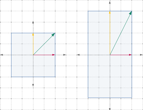
Note that during these transformations, some of the vectors remain on the same line (span) as they were earlier. As shown in the figure,
- The horizontal vector remains unchanged (same direction, same length).
- The vertical vector has same direction, but doubled in length.
- The diagonal vector has changed its angle (direction) as well as length.
Note that, in the above figure, after vertical scaling of +2, every vector’s (except horizontal and vertical ones) direction has changed. These two vectors are special and are the characteristic of this particular transform. Hence, these are called eigenvectors.
An eigenvector is a vector, which after applying the linear transformation, stays in the same span i.e. changes by only a scalar factor.
The eigenvalue is how much the eigenvectors are transformed (stretched or diminished).
- The horizontal vector’s length remains same, thus have an eigenvalue of +1.
- The vertical vectors’ length doubled, thus have an eigenvalue of +2.
Examples
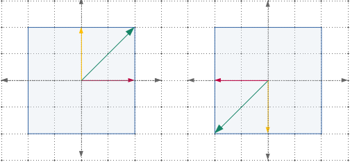
In the same way, the horizontal shear transformation to square gives only one eigenvector (horizontal one) having an eigenvalue of +1.
In 180 degree rotation of square, all vectors are still laying on the same span, but their direction is reversed. Hence, all vectors are eigenvectors, having an eigenvalue of -1.
In case of 3d rotation transformation of cube, the eigenvector gives the axis of rotation.
Mathematics
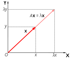
Suppose we have a transformation matrix A and we apply this transformation to vector x. This will be equivalent to stretching (or diminshing) the vector x by a scalar factor λ.
where I is the identity matrix.
The above euqation has a non-zero solution iff the determinant of the matrix (A − λI) is zero i.e.
Evaluating this determinant gives the characteristic polynomial i.e.
\[\text{if } A = \begin{bmatrix} a & b \\ c & d \end{bmatrix}\] \[\begin{vmatrix} \begin{bmatrix} a & b \\ c & d \end{bmatrix} - \begin{bmatrix} \lambda & 0 \\ 0 & \lambda \end{bmatrix} \end{vmatrix} = 0\] \[\lambda ^ 2 - (a+d)\lambda + ad - bc = 0\]The solution of this equation gives the eigvenvalues. Put these eigenvalues in the original expression to get their corresponding eigenvectors.
Why eigenvectors matter for data science: PCA
Eigenvectors and eigenvalues are the foundation of Principal Component Analysis (PCA), one of the most widely used dimensionality reduction techniques. PCA finds a new set of axes, the principal components, that capture the maximum variance in the data. These axes turn out to be the eigenvectors of the covariance matrix of the data.
- The eigenvectors determine the directions of the new feature space (the principal components).
- The eigenvalues determine the magnitude of variance captured by each principal component. Larger eigenvalues mean more variance is explained.
A cumulative eigenvalue plot (scree plot) shows how much of the total variance is captured by the top k components. You typically choose k such that 90–95% of the variance is retained.
PCA can be computed either via eigendecomposition of the covariance matrix or via Singular Value Decomposition (SVD), which is more numerically stable. SVD factorizes a matrix A as:
\[A = USV^T\]where U and V are orthogonal matrices and S is a diagonal matrix of singular values. The columns of V give the principal component directions, and the singular values relate to eigenvalues via \(e_i = \frac{s_i^2}{n-1}\).
References:
Comments