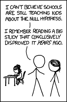
In data science, p-value is used to determine statistical significance of the result. It gives the probability of a statistical model that, when the null hypothesis is true, the statistical summary would be the same or greater than the observed result.
In Simple linear regression, we predict a quantitative response Y on the basis of a singular predictor variable X. It assumes that there is a linear relationship b/w X and Y. Mathematically, it can be written as (we are regressing Y on X):
Here, the model coefficients \(β_{1}\) and \(β_{0}\) represents the slope and intercept in the linear model and \(\epsilon\) is the error term.
We perform Hypothesis tests on the coefficients to check the validity of a claim made about the population. The most common hypothesis tests involves testing the null hypothesis of
\(H_{0}\) : There is no relationship between X and Y
versus the alternate hypothesis
\(H_{a}\) : There is some relationship between X and Y
To test the null hypothesis, we need to determine whether \(\hatβ_{1}\) ,our estimate for \(β_{1}\) , is sufficiently far from zero that we can be confident that \(β_{1}\) is non-zero. We compute t-statistic which measures the number of standard deviations that \(β_{1}\) is away from \(0\).
Consequently, it’s simple to compute the probability of observing any value equal to |t| or larger, assuming \(β_{1} = 0\) (null hypothesis is true). This probability is called p-value. The p-value is defined as the probability, under the null hypothesis \(H_{0}\), of obtaining a result equal to or more extreme than what was actually observed.
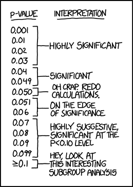
A small p-value indicates that there is an association b/w the predictor and the response. We reject the null hypothesis – i.e. a relationship exists b/w X and Y. Typically, p-value cutoffs for rejecting the null hypothesis is 5% or 1%. Most authors refer to statistically significant as p-value < 0.05 and statistically highly significant as p-value < 0.001 (less than one in a thousand chance of being wrong). The cutoff, \(\alpha\) denotes the significance level of the test.
- “The results are statistically significant” - when the p-value < α.
- “The results are not statistically significant” - when the p-value > α.
Think of a p-value like a detective at a crime scene. The null hypothesis is the assumption of innocence. The detective examines the evidence and asks: “How likely is this evidence if the suspect were innocent?” If the evidence would occur by random chance less than 5% of the time under innocence (p < 0.05), the detective has a strong case to reject innocence. The smaller the p-value, the more compelling the evidence against the null hypothesis. This is not proof of guilt, it is a measure of how surprising the evidence would be under innocence.
No hypothesis test is 100% certain. Because the test is based on probabilities, there is always a chance of drawing an incorrect conclusion. Two types of errors are possible.
- Type I error: It is the false rejection of the null hypothesis i.e. when the null hypothesis is true and you reject it. The probability of making a type I error is α, which is the level of significance you set for your hypothesis test. An α of 0.05 indicates that you are willing to accept a 5% chance that you are wrong when you reject the null hypothesis.
- Type II error: It is the false acceptance of the null hypothesis i.e. when the null hypothesis is false and you fail to reject it. The probability of making a type II error is called β. The quantity (1 - β) is called power, the probability that the test correctly rejects the null hypothesis \(H_{0}\) when a specific alternative hypothesis \(H_{a}\) is true.
Summary
The statistical hypothesis testing process can be summarized in the following steps:
Let’s understand it through an example. A recent study estimated that 20% of all college students in US smoke. The Head of Health Services at Goodheart University suspects that the proportion of smokers may be lower there. In hopes of confirming the claim her claim, she chooses a random sample of 400 Goodheart students, and finds that 70 of them are smokers.
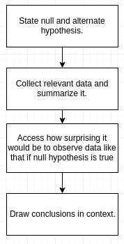
- Stating the claims: There are two claims here:
\(H_{0} :\) The proportion of smokers at Goodheart is 0.20.
\(H_{a} :\) The proportion of smokers at Goodheart is less than 0.20. - Choosing a sample and collecting data: Summarizing the data revealed that the sample proportion of smokers is \(\hat{p} = \frac{70}{400} = 0.175\)
- Assessing the evidence: This is the step where we calculate how likely is it to get data like that observed when \(H_{0}\) true. In other words, we need to find how likely it is that in a random sample of 400 from a poulation, where the proportion of smokers is 0.20, we’ll get a sample proportion as low as \(\hat{p} = 0.175\) (or lower). It turns out that the probability that we’ll get a sample proportion as low as \(\hat{p} = 0.175\) (or lower) in such a sample is roughly 0.106.
- Making conclusions: Do you think that a probability of 0.106 makes our data rare enough (surprising enough) under null hypothesis so that the fact that we did observe it’s enough evidence to reject null hypothesis. Here, p-value = 0.106, which is greater than α (0.05). Thus, we don’t have enough evidene to rejet null hypothesis, \(H_{0}\) i.e. the result is not statistically significant.
Comments
The p-value is often misunderstood as being the probability that the null hypothesis is true.
- Either I reject \(H_{o}\) and accept \(H_{a}\) (when the p-value is smaller than the significance level) or I cannot reject \(H_{o}\) (when the p-value is larger than the significance level).
The second conclusion does not imply that I accept \(H_{o}\), but just that I don’t have enough evidence to reject it.
Related: F-statistic
In multiple regression (with more than one predictor), the F-statistic tests the null hypothesis that all coefficients (except the intercept) are simultaneously zero:
\[F = \frac{\text{variation explained by the model}}{\text{variation not explained by the model}}\]A large F-statistic with a small p-value tells you that at least one predictor in the model is significant.
References:
Comments